KANs take longer to train, but they have the advantages of being far more interpretable and faster to use, because they find an analytical equation as a final model, which is typically just a series of polynomials.
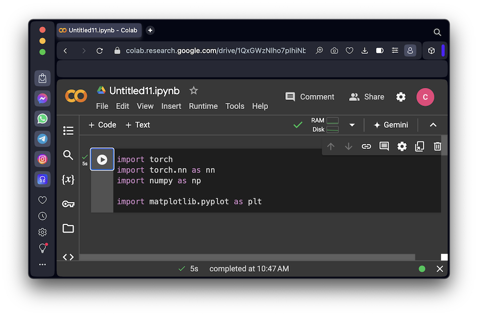
https://colab.research.google.com/If you see a blue "Sign In" button at the top right, click it and log into a Google account.
From the menu, click File, "New notebook".
import torch
import torch.nn as nn
import numpy as np

import matplotlib.pyplot as plt
For this example, we'll use 20 control points evenly spaced in the range from x = -1 to x = 1.
Execute these commands:
grid = torch.linspace(-1, 1, steps=20)
x = torch.linspace(-1, 1, steps=1000) # we take the entire domain to plot the basis function as a function of x
# Reshape so that each x can be compared to each control point
grid_ = grid.unsqueeze(dim=0)
x_ = x.unsqueeze(dim=1)
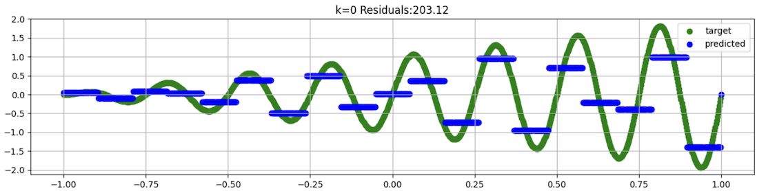
k = 0 # This gives us basis functions for order 0
value1 = (x_ >= grid_[:,:-1]) * (x_ < grid_[:, 1:])
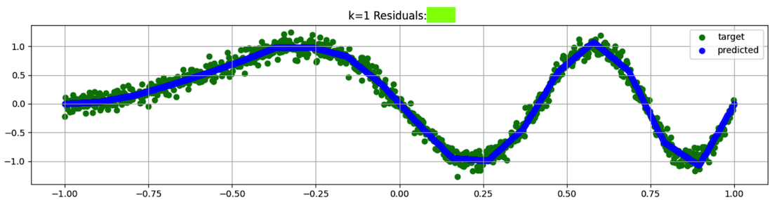
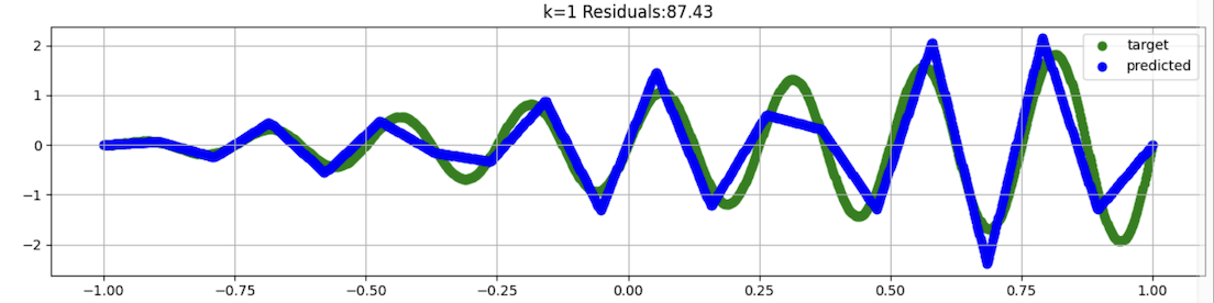
k = 1 # This gives us basis functions for order 1
value21 = (x_ - grid_[:, :-(k+1)]) / (grid_[:, 1:-k] - grid_[:, :-(k+1)]) * value1[:, :-1]
value22 = (grid_[:, (k+1):] - x_) / (grid_[:, (k+1):] - grid_[:, 1:-k]) * value1[:, 1:]
value2 = value21 + value22
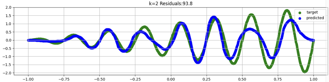
k = 2 # This gives us basis functions for order 2
value31 = (x_ - grid_[:, :-(k+1)]) / (grid_[:, 1:-k] - grid_[:, :-(k+1)]) * value2[:, :-1]
value32 = (grid_[:, (k+1):] - x_) / (grid_[:, (k+1):] - grid_[:, 1:-k]) * value2[:, 1:]
value3 = value31 + value32
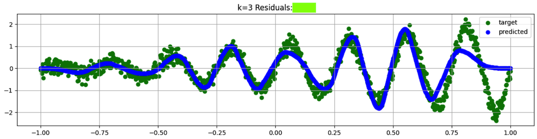
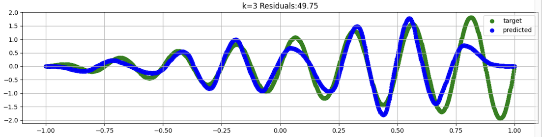
k = 3 # This gives us basis functions for order 3
value41 = (x_ - grid_[:, :-(k+1)]) / (grid_[:, 1:-k] - grid_[:, :-(k+1)]) * value3[:, :-1]
value42 = (grid_[:, (k+1):] - x_) / (grid_[:, (k+1):] - grid_[:, 1:-k]) * value3[:, 1:]
value4 = value41 + value42
fn = lambda x: torch.sin(torch.pi * (x+1)* 8)*(x+1)
all_basis = [(value1 * 1.0, 'k=0'), (value2, 'k=1'), (value3, 'k=2'), (value4, 'k=3')]
fig, axs = plt.subplots(nrows=len(all_basis), figsize=(15, 15), dpi=100)
for i in range(len(all_basis)):
ax = axs[i]
value, label = all_basis[i]
y_correct = fn(x)
coeff = torch.linalg.lstsq(value, y_correct).solution # find the coefficients
y_pred = torch.einsum('i, ji -> j', coeff, value) # use these coefficients to evaluate y
residuals = 0
for k in range(150, len(y_correct) - 150):
residuals += (y_pred[k] - y_correct[k]) ** 2
ax.scatter(x, y_correct, color='green', label='target')
ax.scatter(x, y_pred, color='blue', label="predicted")
ax.grid()
ax.set_title(f"{label}" + " Residuals:" + str(round(residuals.item(), 2)))
ax.legend()
This approximates the curve as a series of horizontal lines, as shown below.
This is a very sloppy fit, missing a lot of the actual curves in the data.
Notice the Residuals value: this is the sum of the squared errors, for the center portion of the data, to exclude problems near the edges.
This is better than order 0, with a smaller Residuals value, but still misses some of the curves, as shown below.
This fit still misses badly on the right side of the chart, as shown below.
This is a better fit, with the lowest Residials value of all, as shown below.
The bad errors on the right side occur because there aren't any control points for x > 1, so there are errors at the boundary.
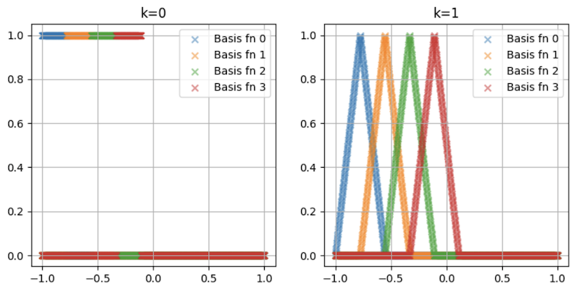
To see the basis functions, execute these commands:
# Here, we define the control points.
grid = torch.linspace(-1, 1, steps=10)
# we take the entire domain to plot the basis function as a function of x
x = torch.linspace(-1, 1, steps=1000)
# Reshape so that each x can be compared to each control point
grid_ = grid.unsqueeze(dim=0)
x_ = x.unsqueeze(dim=1)
# Base case
k = 0
value1 = (x_ >= grid_[:,:-1]) * (x_ < grid_[:, 1:])
# Other cases
k = 1 # This gives us basis functions for order 1
value21 = (x_ - grid_[:, :-(k+1)]) / (grid_[:, 1:-k] - grid_[:, :-(k+1)]) * value1[:, :-1]
value22 = (grid_[:, (k+1):] - x_) / (grid_[:, (k+1):] - grid_[:, 1:-k]) * value1[:, 1:]
value2 = value21 + value22
k = 2 # This gives us basis functions for order 2
value31 = (x_ - grid_[:, :-(k+1)]) / (grid_[:, 1:-k] - grid_[:, :-(k+1)]) * value2[:, :-1]
value32 = (grid_[:, (k+1):] - x_) / (grid_[:, (k+1):] - grid_[:, 1:-k]) * value2[:, 1:]
value3 = value31 + value32
k = 3 # This gives us basis functions for order 3
value41 = (x_ - grid_[:, :-(k+1)]) / (grid_[:, 1:-k] - grid_[:, :-(k+1)]) * value3[:, :-1]
value42 = (grid_[:, (k+1):] - x_) / (grid_[:, (k+1):] - grid_[:, 1:-k]) * value3[:, 1:]
value4 = value41 + value42
fig, axs = plt.subplots(ncols=2, nrows=2, figsize=(9, 9), dpi=100)
n_basis_to_plot = 4
all_basis = [(value1, 'k=0'), (value2, 'k=1'), (value3, 'k=2'), (value4, 'k=3')]
for i in range(4):
ax = axs[i // 2, i % 2]
value, label = all_basis[i]
for idx in range(value.shape[-1])[:n_basis_to_plot]:
ax.scatter(x, value[:, idx], marker='x', label=f"Basis fn {idx}", alpha=0.5)
ax.grid()
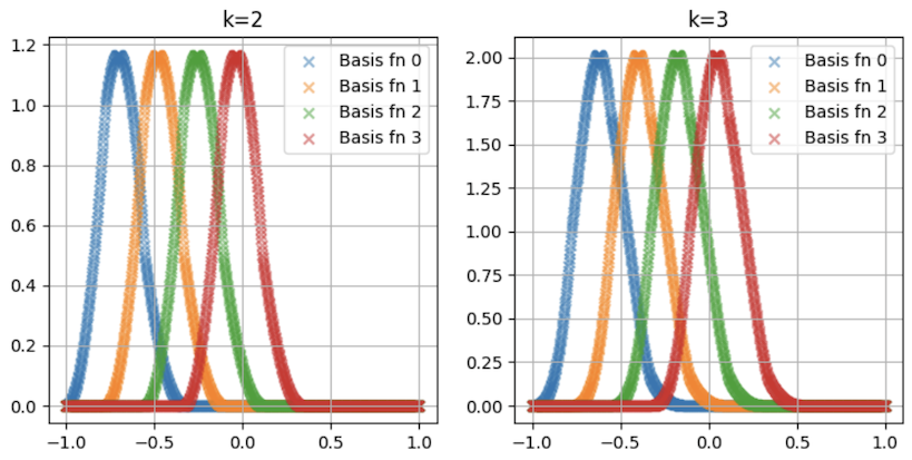
ax.set_title(label)
ax.legend()
Order zero uses basis functions that are 1 near the control point, and 0 elsewhere.
For order 1, the basis functions are pyramids with linear sides, peaking at the location of the control points.
This means that the model can be controlled and adjusted more easily and reliably. KAN models resist the problem of "catastrophic forgetting", when neural nets that are fine-tuned on new data forget what they learned from the old data.
ML 181.1: Adding Noise (5 pts)
Repace the fn definition with this:Fit the data with B-splines as you did before.The flag is covered by a green rectangle in the image below.
ML 181.2: FM (5 pts)
Repace the fn definition with this:Fit the data with B-splines.The flag is covered by a green rectangle in the image below.
ML 181.3: Wild (5 pts)
Repace the fn definition with this:Use a grid with 50 steps rather than 20.Fit the data with B-splines.
The flag is covered by a green rectangle in the image below.
Posted 8-8-24
Flag 1 answer updated 5-16-25