This is an old, classic, method which doesn't need neural networks. However, as you will see, it often produces poor results, especially if the power is too high.
https://colab.research.google.com/If you see a blue "Sign In" button at the top right, click it and log into a Google account.
From the menu, click File, "New notebook".
Execute this code:
import numpy as np
import matplotlib.pyplot as plt

# Specify seed to make random numbers reproducible
np.random.seed(0)

# Generate some noisy data
x = np.linspace(0, 10, 20)
y = 2 * x**2 + 3 * x + 1 + np.random.normal(0, 10, 20)

degree = 2

# Fit a polynomial
coeffs, res, _, _, _ = np.polyfit(x, y, degree, full=True)

# Create a polynomial function using the coefficients
poly_func = np.poly1d(coeffs)

# Generate y values for the fitted curve
y_fit = poly_func(x)

# Plot the original data and the fitted curve
plt.scatter(x, y, label="Data")
plt.plot(x, y_fit, label="Fitted Curve", color="red")

plt.title("Polynomial of degree "+ str(degree) + \
          " Residuals: " + str(round(res[0], 2)))
plt.xlabel("x")
plt.ylabel("y")
plt.legend()
plt.show()
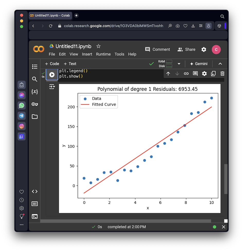
Notice the "Residuals" value--this is the sum of the squared errors. The lower this value, the better the fit to the data.
As shown below, it fits the best line possible through the data, but it has systematic errors: the dots are all below the line in the middle, and above it at the ends. This is unavoidable because the dots follow a curved parabola, so no straight line can model that behavior.
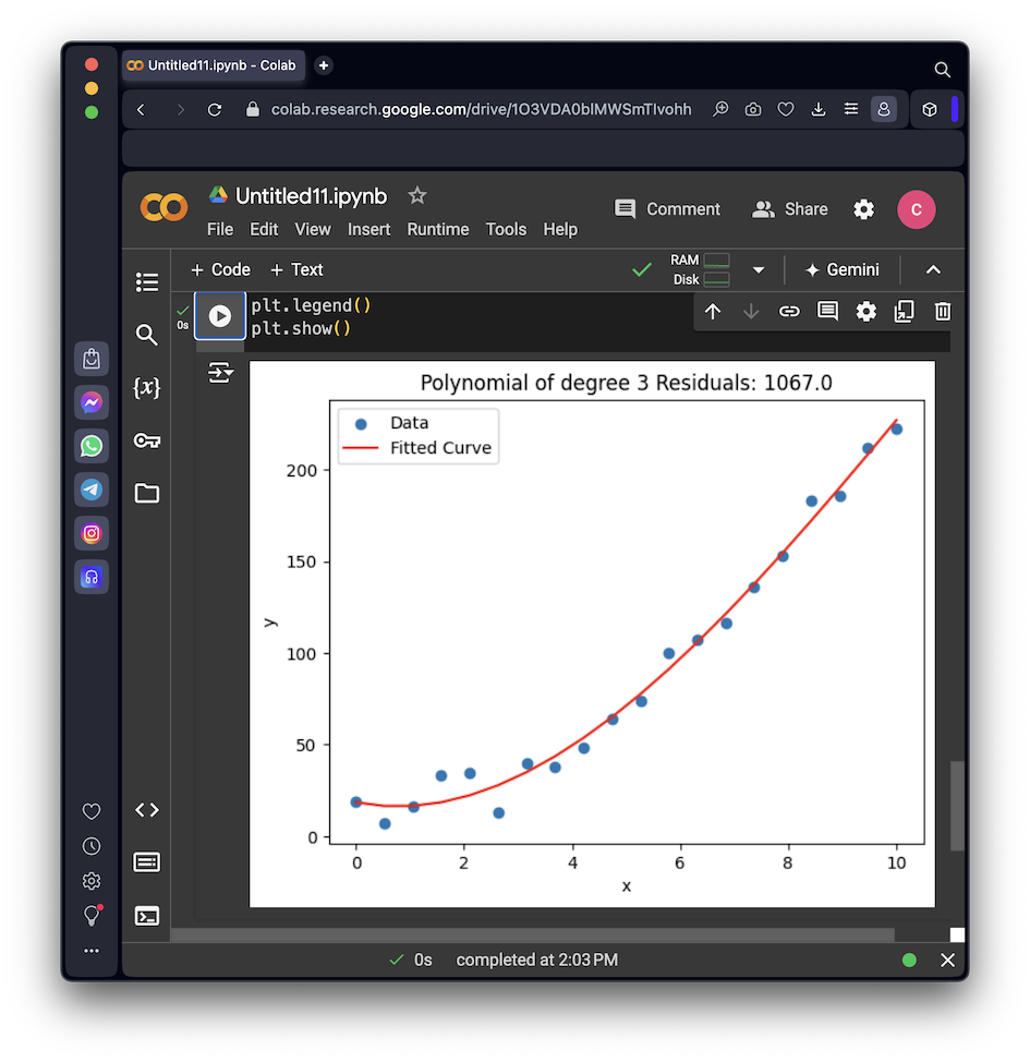
Notice that the Residuals is much larger, indicating that this is an inferior fit to the data.
As shown below, the fit still looks good, and the Residuals are lower than the fit with degree=2. But we know the underlying trend is a parabola, so the 3rd-order term must be fitting the noise, not the trend.
To detect this problem, we'd need a separate set of test data to evaluate the fit, with the same trend but different noise.
ML 180.1: Degree Nine (5 pts)
Change the code above to use degree==9.As shown below, the fit follows the noise more closely.
The flag is covered by a green rectangle in the image below.
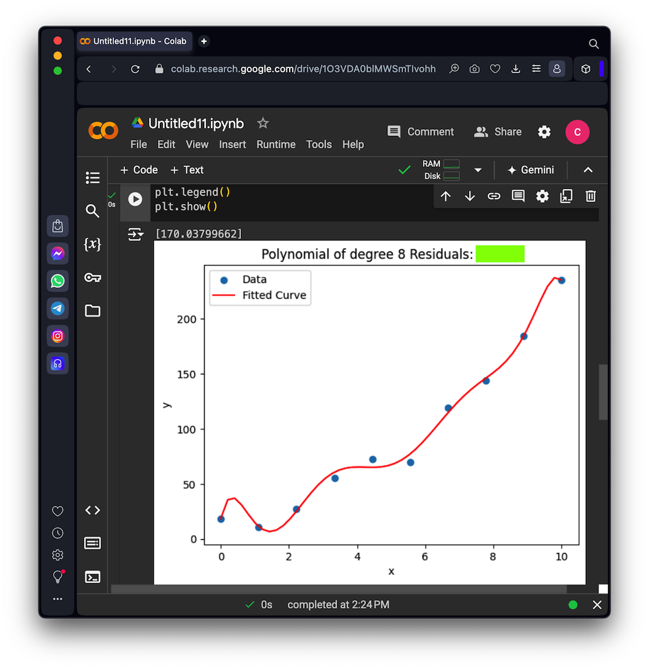
ML 180.2: Fewer Points (10 pts)
In the code above, this line creates a list of X values going from 0 to 10, with a total of 20 points:Change that line to this line, which produces only 10 points:Fit the data with degree=8.
The flag is covered by a green rectangle in the image below.
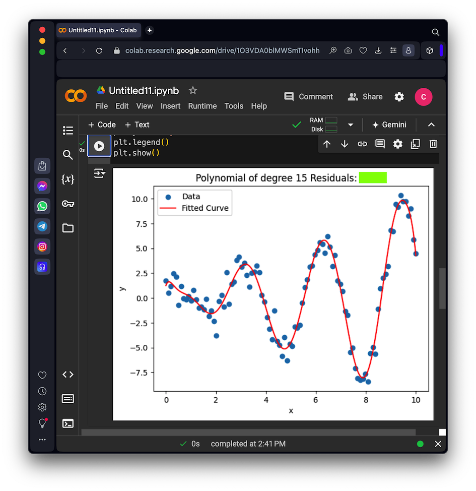
ML 180.3: Complex Curve (15 pts)
Instead of a parabola, use this data, which produces 100 points on a complex curve:You will need to change x to also have 100 points.Fit a 15th degree polynomial.
The flag is covered by a green rectangle in the image below.
Posted 5-21-24
Tip to enable inline suggestions added 7-24-24
Instructions corrected for flags 2 and 3 5-12-26