https://colab.research.google.com/If you see a blue "Sign In" button at the top right, click it and log into a Google account.
From the menu, click File, "New notebook".
import random
random.seed(999)
print("Dimensions \t Edge points out of 1000")
for dimensions in [2,3,10,30,100,300,1000,3000,10000]:
  edge_points = 0
  for p in range(1000):
    on_edge = 0
    for x in range(dimensions):
      if random.random() < 0.01:
        on_edge = 1
    edge_points += on_edge
  print(dimensions, "\t\t", edge_points)
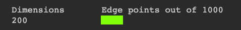
Flag ML 115.1: 200 Dimensions (5 pts)
Repeat the process above, but use 3000 samples and test only 200 dimensions.Leave the random.seed at 999, to ensure that you get the expected flag value.
The flag is covered by a green rectangle in the image below.
import random, math
random.seed(999)
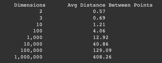
print("Dimensions \t Avg Distance Between Points")
for dimensions in [2, 3, 10, 100, 1_000, 10_000, 100_000, 1_000_000]:
total_distance = 0
for p in range(100):
dist2 = 0
for x in range(dimensions):
dist2 += (random.random() - random.random())**2
total_distance += math.sqrt(dist2)
formatted_dimensions = "{:,}".format(dimensions)
print(formatted_dimensions.rjust(9), "\t\t", "{:.2f}".format(total_distance/100.0))
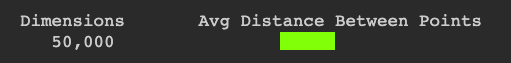
Flag ML 115.2: 50,000 Dimensions (5 pts)
Repeat the process above, but use 300 pairs of points and test only 50,000 dimensions.Make sure you divide the total distance by 300 to get the average distance.
Leave the random.seed at 999, to ensure that you get the expected flag value.
The flag is covered by a green rectangle in the image below.
from sklearn.datasets import fetch_openml
import numpy as np

mnist = fetch_openml('mnist_784', as_frame=False, parser="auto")
X_train, y_train = mnist.data[:60_000], mnist.target[:60_000]
X_test, y_test = mnist.data[60_000:], mnist.target[60_000:]

import matplotlib.pyplot as plt

def plot_digit(image_data):
    image = image_data.reshape(28, 28)
    plt.imshow(image, cmap="binary")
    plt.axis("off")

plt.figure(figsize=(4, 4))
for idx, image_data in enumerate(X_train[:16]):
    plt.subplot(4, 4, idx + 1)
    plot_digit(image_data)
plt.subplots_adjust(wspace=0, hspace=0)
plt.show()
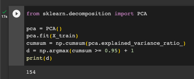
Execute these commands to find the number of dimensions needed to fit 95% of the variance:
from sklearn.decomposition import PCA

pca = PCA()
pca.fit(X_train)
cumsum = np.cumsum(pca.explained_variance_ratio_)
d = np.argmax(cumsum >= 0.95) + 1
print(d)
Flag ML 115.3: 99% of the Variance (5 pts)
Repeat the process above, but explain 99% of the variance.The flag is the number of dimensions required.
This model uses RandomizedSearchCV to find a good combination of hyperparameters for both PCA and the random forest classifier. The only two hyperparameters tested are pca__n_components and randomforestclassifier__n_estimators.
To speed things up, we use only the 100 training images and only perform 10 iterations.
from sklearn.ensemble import RandomForestClassifier
from sklearn.model_selection import RandomizedSearchCV
from sklearn.pipeline import make_pipeline
from sklearn.metrics import accuracy_score

clf = make_pipeline(PCA(random_state=42),
                    RandomForestClassifier(random_state=42))
param_distrib = {
    "pca__n_components": np.arange(10, 80),
    "randomforestclassifier__n_estimators": np.arange(50, 500)
}
rnd_search = RandomizedSearchCV(clf, param_distrib, n_iter=10, cv=3,
                                random_state=42)
rnd_search.fit(X_train[:1000], y_train[:1000])

print(rnd_search.best_params_)

y_pred = rnd_search.predict(X_test)
accuracy_score = accuracy_score(y_pred,y_test)
print(accuracy_score)
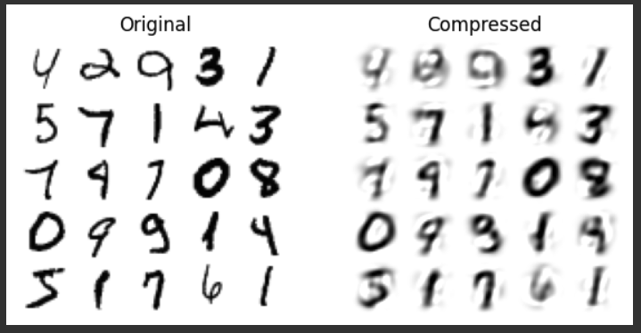
pca = PCA(n_components=23)
X_reduced = pca.fit_transform(X_train, y_train)
X_recovered = pca.inverse_transform(X_reduced)

plt.figure(figsize=(7, 4))
for idx, X in enumerate((X_train[::2100], X_recovered[::2100])):
    plt.subplot(1, 2, idx + 1)
    plt.title(["Original", "Compressed"][idx])
    for row in range(5):
        for col in range(5):
            plt.imshow(X[row * 5 + col].reshape(28, 28), cmap="binary",
                       vmin=0, vmax=255, extent=(row, row + 1, col, col + 1))
            plt.axis([0, 5, 0, 5])
            plt.axis("off")
Flag ML 115.4: 99% of the Variance (5 pts)
Repeat the process above, but change n_iter from 10 to 3, and change the number of training samples used from 1000 to 3000.The flag is the number of dimensions used, covered by a green rectangle in the image below.
Posted 10-6-23
Video added 10-21-23
Title of flag 2 fixed 7-24-24