https://colab.research.google.com/If you see a blue "Sign In" button at the top right, click it and log into a Google account.
From the menu, click File, "New notebook".
import matplotlib.pyplot as plt
from sklearn.datasets import make_moons
from sklearn.model_selection import train_test_split
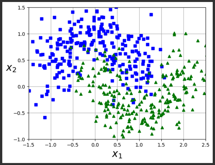
X, y = make_moons(n_samples=500, noise=0.30, random_state=42)
X_train, X_test, y_train, y_test = train_test_split(X, y, random_state=42)
def plot_dataset(X, y, axes):
plt.plot(X[:, 0][y==0], X[:, 1][y==0], "bs")
plt.plot(X[:, 0][y==1], X[:, 1][y==1], "g^")
plt.axis(axes)
plt.grid(True, which='both')
plt.xlabel(r"$x_1$", fontsize=20)
plt.ylabel(r"$x_2$", fontsize=20, rotation=0)
plot_dataset(X, y, [-1.5, 2.5, -1, 1.5])
plt.show()
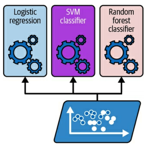
A Support Vector Machine uses a line to separate classes
A Random Forest is an ensemble of decision trees (100 trees by default for sklearn's RandomForestClassifier).
Execute these commands to create a voting classifier containint those three predictors:
from sklearn.ensemble import RandomForestClassifier, VotingClassifier
from sklearn.linear_model import LogisticRegression
from sklearn.svm import SVC
voting_clf = VotingClassifier(
estimators=[
('lr', LogisticRegression(random_state=42)),
('rf', RandomForestClassifier(random_state=42)),
('svc', SVC(random_state=42))
]
)
voting_clf.fit(X_train, y_train)
VotingClassifier(estimators=[('lr', LogisticRegression(random_state=42)),
('rf', RandomForestClassifier(random_state=42)),
('svc', SVC(random_state=42))])
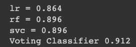
for name, clf in voting_clf.named_estimators_.items():
print(name, "=", clf.score(X_test, y_test))
print("Voting Classifier", voting_clf.score(X_test, y_test))
In soft voting, each predictor outputs a probability, and those probabilities are averaged. This makes use of more information from each predictor, and should therefore be more accurate.
To implement soft voting, execute these commands:
voting_clf.voting = "soft"
voting_clf.named_estimators["svc"].probability = True
voting_clf.fit(X_train, y_train)

print("Soft Voting Classifier", voting_clf.score(X_test, y_test))
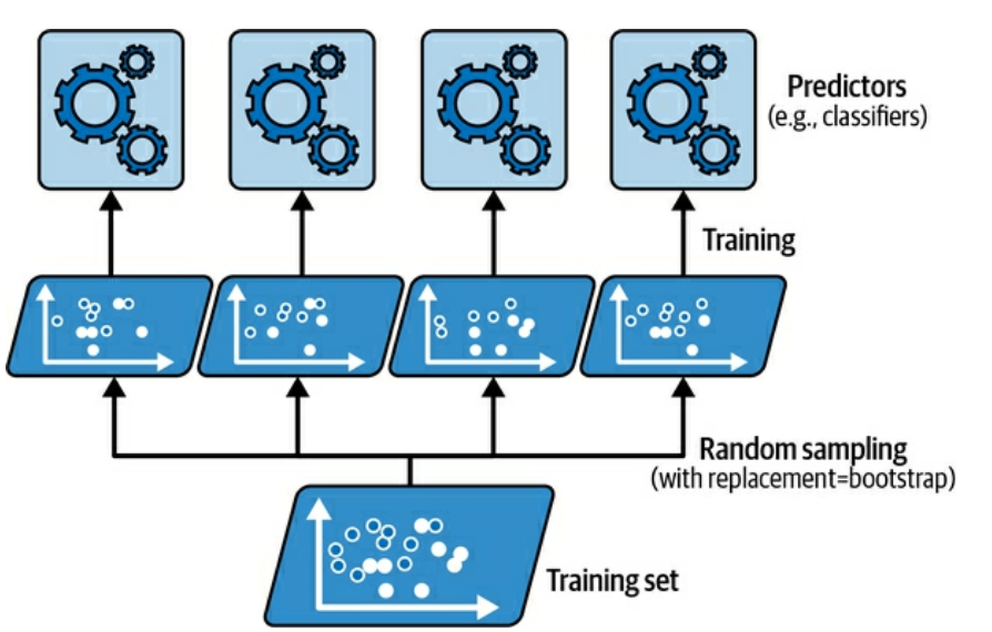
Execute these commands to create the Bagging classifier using a forest with 500 trees:
from sklearn.ensemble import BaggingClassifier
from sklearn.tree import DecisionTreeClassifier
from sklearn.metrics import accuracy_score
import numpy as np
bag_clf = BaggingClassifier(DecisionTreeClassifier(), n_estimators=500,
max_samples=100, n_jobs=-1, random_state=42)
bag_clf.fit(X_train, y_train)
BaggingClassifier(estimator=DecisionTreeClassifier(), max_samples=100,
n_estimators=500, n_jobs=-1, random_state=42)
def plot_decision_boundary(clf, X, y, alpha=1.0):
axes=[-1.5, 2.4, -1, 1.5]
x1, x2 = np.meshgrid(np.linspace(axes[0], axes[1], 100),
np.linspace(axes[2], axes[3], 100))
X_new = np.c_[x1.ravel(), x2.ravel()]
y_pred = clf.predict(X_new).reshape(x1.shape)
plt.contourf(x1, x2, y_pred, alpha=0.3 * alpha, cmap='Wistia')
plt.contour(x1, x2, y_pred, cmap="Greys", alpha=0.8 * alpha)
colors = ["#78785c", "#c47b27"]
markers = ("o", "^")
for idx in (0, 1):
plt.plot(X[:, 0][y == idx], X[:, 1][y == idx],
color=colors[idx], marker=markers[idx], linestyle="none")
plt.axis(axes)
plt.xlabel(r"$x_1$")
plt.ylabel(r"$x_2$", rotation=0)
tree_clf = DecisionTreeClassifier(random_state=42)
tree_clf.fit(X_train, y_train)
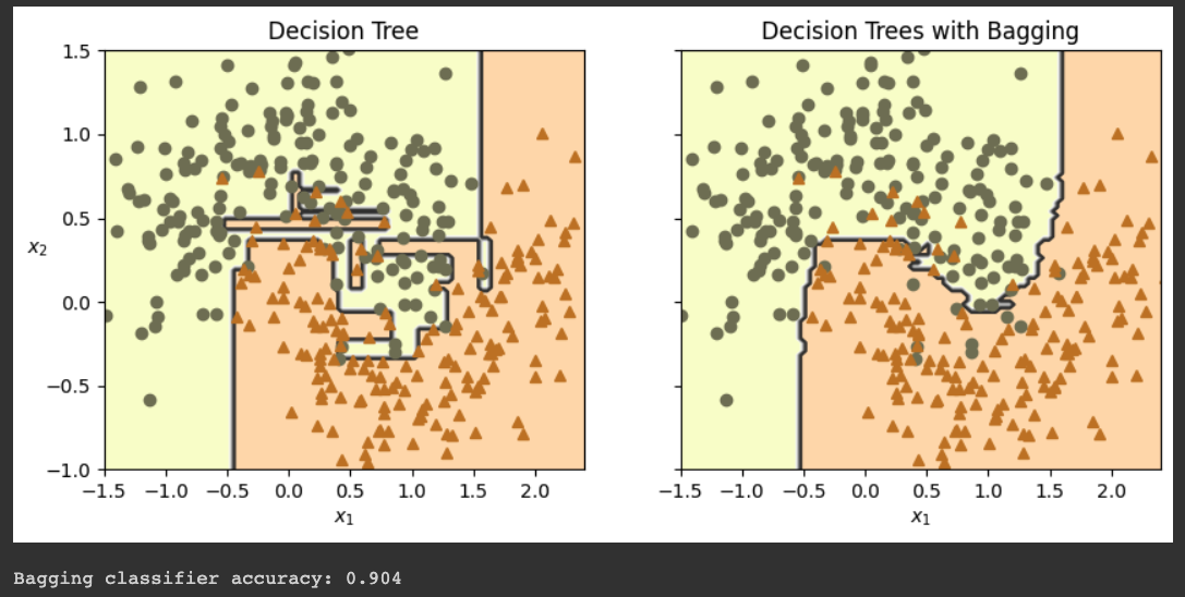
fig, axes = plt.subplots(ncols=2, figsize=(10, 4), sharey=True)
plt.sca(axes[0])
plot_decision_boundary(tree_clf, X_train, y_train)
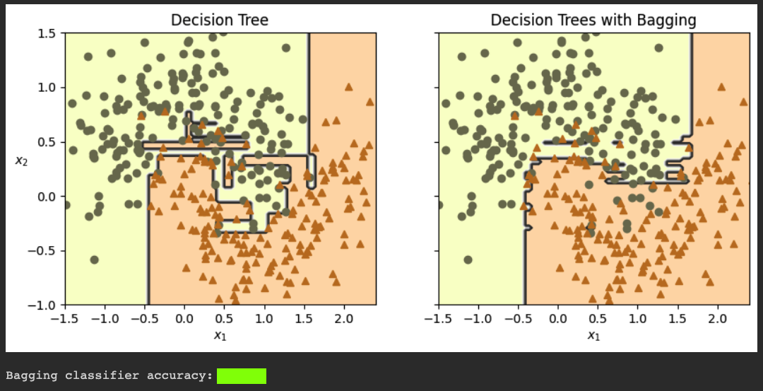
plt.title("Decision Tree")
plt.sca(axes[1])
plot_decision_boundary(bag_clf, X_train, y_train)
plt.title("Decision Trees with Bagging")
plt.ylabel("")
plt.show()
y_pred = bag_clf.predict(X_test)
print()
print("Bagging classifier accuracy:", accuracy_score(y_test, y_pred))
Flag ML 114.1: 5 Trees (5 pts)
Repeat the process above, but change n_estimators in the most recent block of code from 500 to 5 both places it appears. The model has more overfitting, as shown below.The flag is the accuracy of the prediction, covered by a green rectangle in the image below.
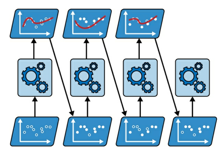
The algorithm increases the weight of instances that were incorrectly predicted by the previous predictor, as shown below.
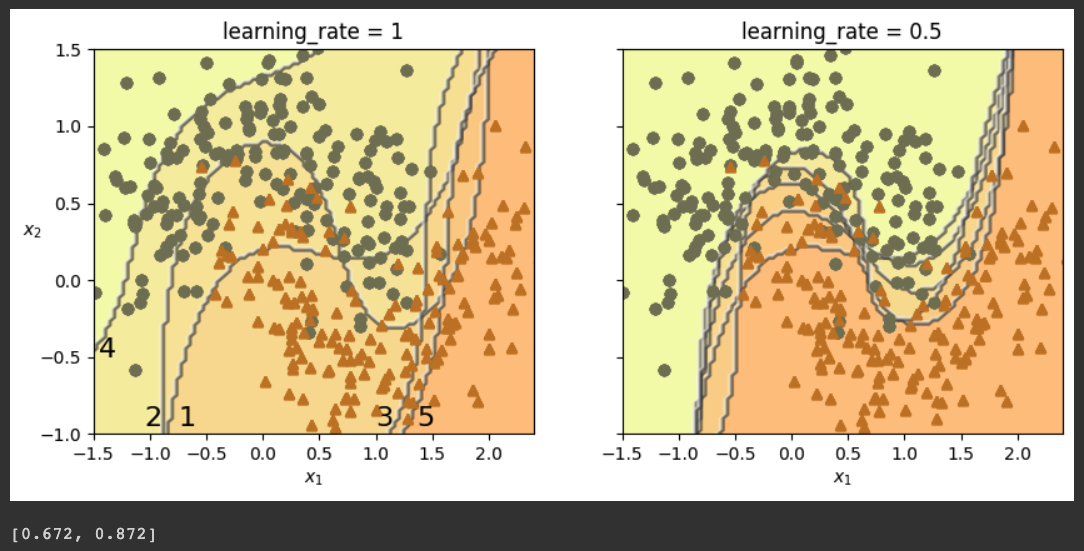
Execute these commands to perform 5 iterations of AdaBoost using a jighly regularized SVM classifier with an RBF kernel:
m = len(X_train)

accuracy = [0,0]

fig, axes = plt.subplots(ncols=2, figsize=(10, 4), sharey=True)
for subplot, learning_rate in ((0, 1), (1, 0.5)):
    sample_weights = np.ones(m) / m
    plt.sca(axes[subplot])
    for i in range(5):
        svm_clf = SVC(C=0.2, gamma=0.6, random_state=42)
        svm_clf.fit(X_train, y_train, sample_weight=sample_weights * m)
        y_pred = svm_clf.predict(X_train)

        error_weights = sample_weights[y_pred != y_train].sum()
        r = error_weights / sample_weights.sum()  # equation 7-1
        alpha = learning_rate * np.log((1 - r) / r)  # equation 7-2
        sample_weights[y_pred != y_train] *= np.exp(alpha)  # equation 7-3
        sample_weights /= sample_weights.sum()  # normalization step

        plot_decision_boundary(svm_clf, X_train, y_train, alpha=0.4)
        plt.title(f"learning_rate = {learning_rate}")
    if subplot == 0:
        plt.text(-0.75, -0.95, "1", fontsize=16)
        plt.text(-1.05, -0.95, "2", fontsize=16)
        plt.text(1.0, -0.95, "3", fontsize=16)
        plt.text(-1.45, -0.5, "4", fontsize=16)
        plt.text(1.36,  -0.95, "5", fontsize=16)
    else:
        plt.ylabel("")
    accuracy[subplot] = svm_clf.score(X_test, y_test)

plt.show()

print()
print(accuracy)
The plot on the right shows the result with a slower learning rate--converging on a better solution--87% accuracy.
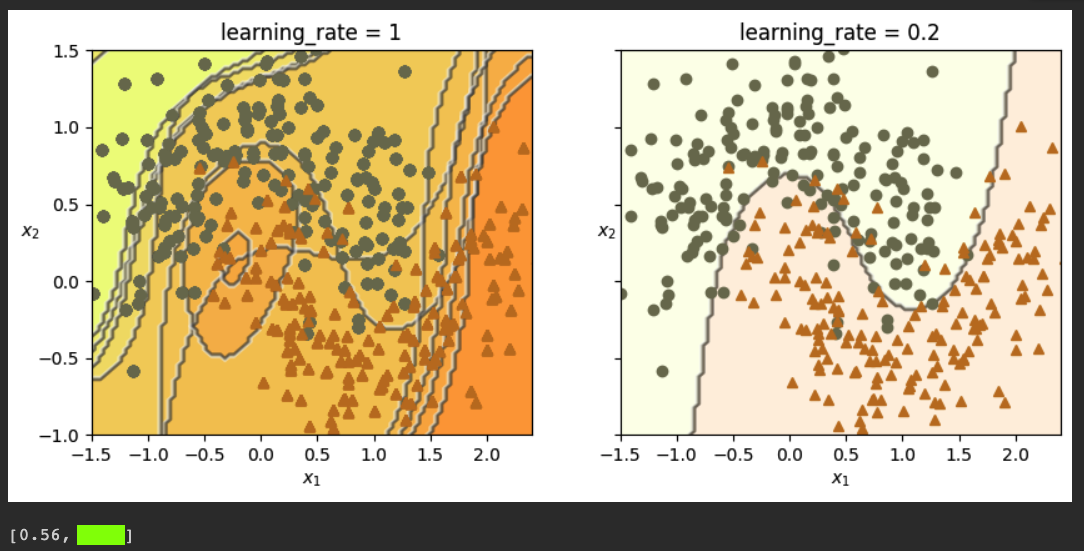
Flag ML 114.2: Ten Cycles (10 pts)
Repeat the process above, but change learning_rate from 0.5 to 0.2, and run it for 10 iterations, not 5. (I removed the boundaries from the right plot, showing only the last one, but you don't need to do that to get the flag.)The flag is covered by a green rectangle in the image below.
Posted 10-1-23
Video added 10-21-23
Descriptions of the three classifier types added 6-28-24
"base_estimator" renamed to "estimator" 12-12-24