https://github.com/pralab/secml/blob/master/tutorials/06-MNIST_dataset.ipynb
Jupyter Notebook Server
This project uses the SecML library, which hasn't been updated since 2023. It no longer works in Google Colab. Instead, you need to use a local virtual machine running an older Jupyter Notebook.See project ML 107 to see how to download and run that machine.
import secml
from secml.data.loader import CDataLoaderMNIST
loader = CDataLoaderMNIST()
random_state = 999
n_tr = 100 # Number of training set samples
n_val = 500 # Number of validation set samples
n_ts = 500 # Number of test set samples
digits = (5, 9)
tr_val = loader.load('training', digits=digits, num_samples=n_tr + n_val)
ts = loader.load('testing', digits=digits, num_samples=n_ts)
# Split in training and validation set
tr = tr_val[:n_tr, :]
val = tr_val[n_tr:, :]
# Normalize the features in `[0, 1]`
tr.X /= 255
val.X /= 255
ts.X /= 255
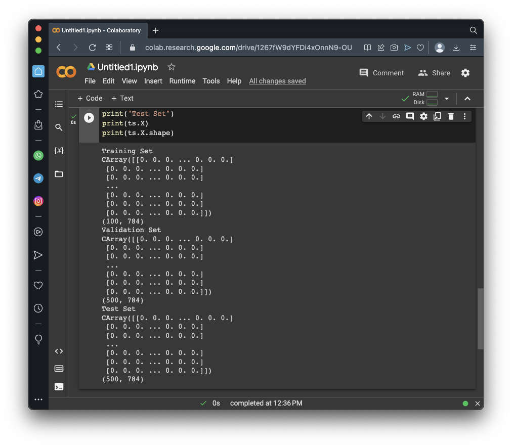
print("Training Set")
print(tr.X)
print(tr.X.shape)
print("Validation Set")
print(val.X)
print(val.X.shape)
print("Test Set")
print(ts.X)
print(ts.X.shape)
from secml.figure import CFigure
# Only required for visualization in notebooks
%matplotlib inline
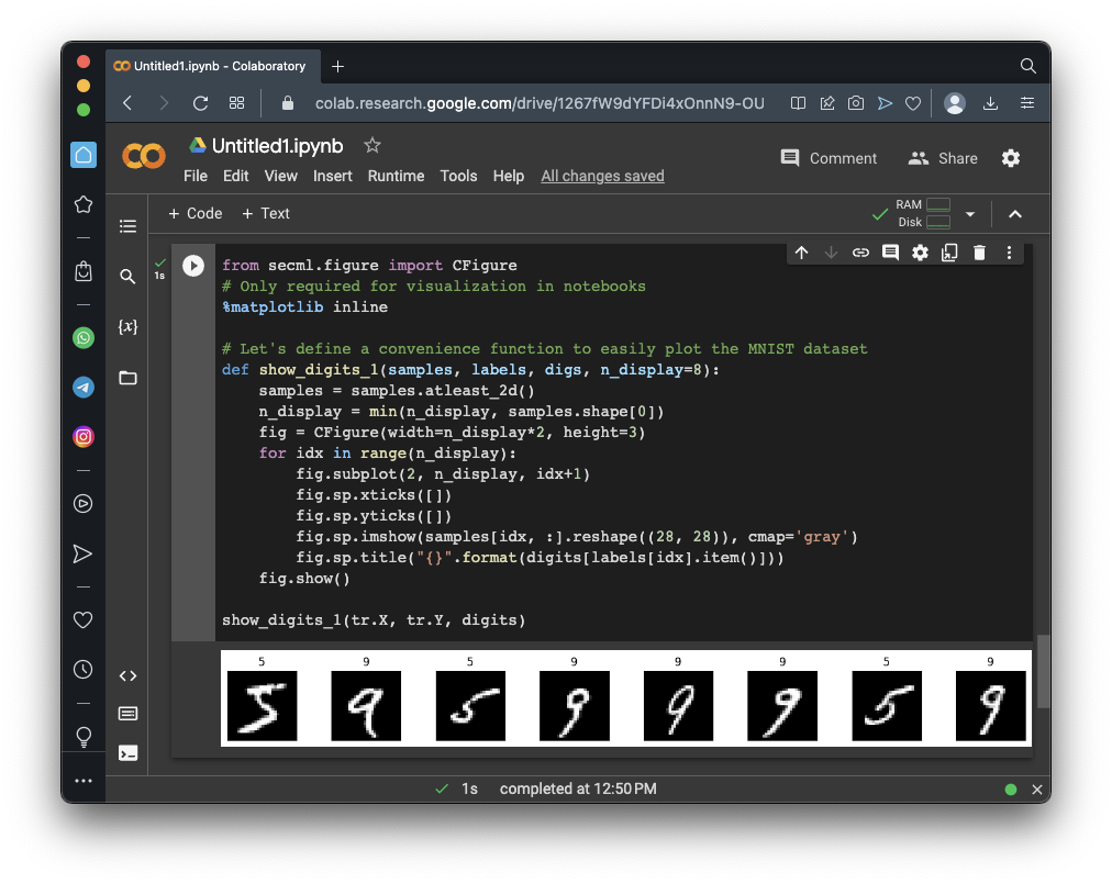
# Let's define a convenience function to easily plot the MNIST dataset
def show_digits_1(samples, labels, digs, n_display=8):
samples = samples.atleast_2d()
n_display = min(n_display, samples.shape[0])
fig = CFigure(width=n_display*2, height=3)
for idx in range(n_display):
fig.subplot(2, n_display, idx+1)
fig.sp.xticks([])
fig.sp.yticks([])
fig.sp.imshow(samples[idx, :].reshape((28, 28)), cmap='gray')
fig.sp.title("{}".format(digits[labels[idx].item()]))
fig.show()
show_digits_1(tr.X, tr.Y, digits)
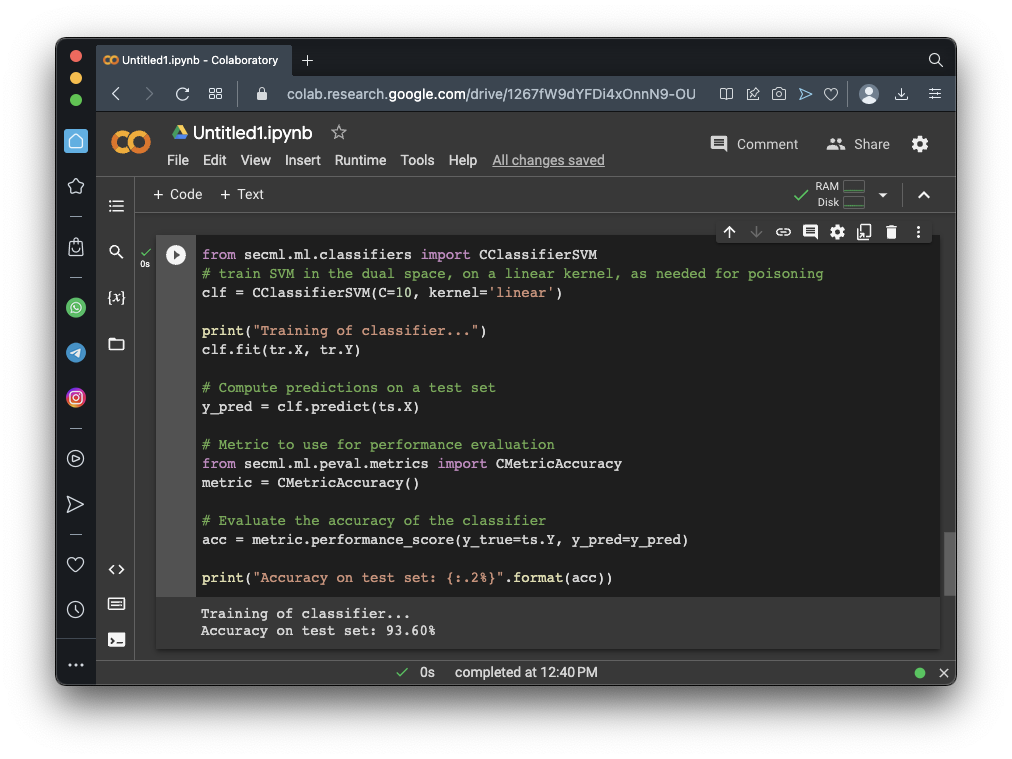
from secml.ml.classifiers import CClassifierSVM
# train SVM in the dual space, on a linear kernel, as needed for poisoning
clf = CClassifierSVM(C=10, kernel='linear')

print("Training of classifier...")
clf.fit(tr.X, tr.Y)

# Compute predictions on a test set
y_pred = clf.predict(ts.X)

# Metric to use for performance evaluation
from secml.ml.peval.metrics import CMetricAccuracy
metric = CMetricAccuracy()

# Evaluate the accuracy of the classifier
acc = metric.performance_score(y_true=ts.Y, y_pred=y_pred)

print("Accuracy on test set: {:.2%}".format(acc))
# For simplicity, let's attack a subset of the test set
attack_ds = ts[:25, :]
noise_type = 'l2' # Type of perturbation 'l1' or 'l2'
dmax = 2.5 # Maximum perturbation
lb, ub = 0., 1. # Bounds of the attack space. Can be set to `None` for unbounded
y_target = None # None if `error-generic` or a class label for `error-specific`
# Should be chosen depending on the optimization problem
solver_params = {
'eta': 0.5,
'eta_min': 2.0,
'eta_max': None,
'max_iter': 100,
'eps': 1e-6
}
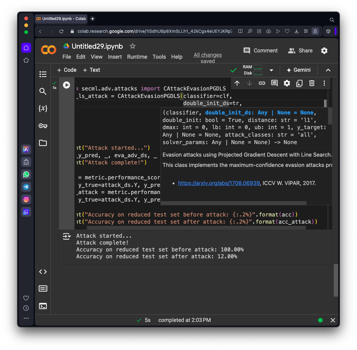
from secml.adv.attacks import CAttackEvasionPGDLS
pgd_ls_attack = CAttackEvasionPGDLS(classifier=clf,
double_init_ds=tr,
distance=noise_type,
dmax=dmax,
solver_params=solver_params,
y_target=y_target)
print("Attack started...")
eva_y_pred, _, eva_adv_ds, _ = pgd_ls_attack.run(attack_ds.X, attack_ds.Y)
print("Attack complete!")
acc = metric.performance_score(
y_true=attack_ds.Y, y_pred=clf.predict(attack_ds.X))
acc_attack = metric.performance_score(
y_true=attack_ds.Y, y_pred=eva_y_pred)
print("Accuracy on reduced test set before attack: {:.2%}".format(acc))
print("Accuracy on reduced test set after attack: {:.2%}".format(acc_attack))
from secml.figure import CFigure
# Only required for visualization in notebooks
%matplotlib inline
# Let's define a convenience function to easily plot the MNIST dataset
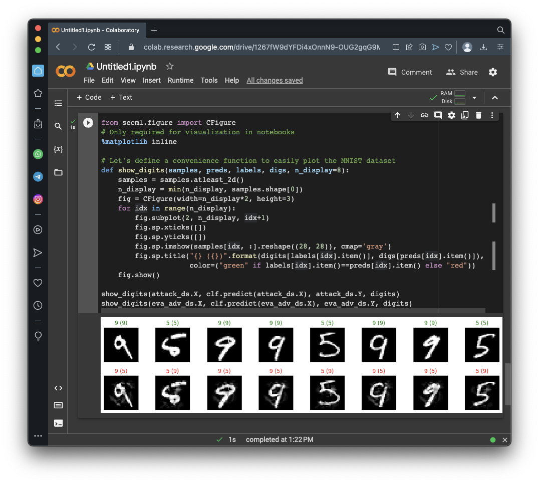
def show_digits(samples, preds, labels, digs, n_display=8):
samples = samples.atleast_2d()
n_display = min(n_display, samples.shape[0])
fig = CFigure(width=n_display*2, height=3)
for idx in range(n_display):
fig.subplot(2, n_display, idx+1)
fig.sp.xticks([])
fig.sp.yticks([])
fig.sp.imshow(samples[idx, :].reshape((28, 28)), cmap='gray')
fig.sp.title("{} ({})".format(digits[labels[idx].item()], digs[preds[idx].item()]),
color=("green" if labels[idx].item()==preds[idx].item() else "red"))
fig.show()
show_digits(attack_ds.X, clf.predict(attack_ds.X), attack_ds.Y, digits)
show_digits(eva_adv_ds.X, clf.predict(eva_adv_ds.X), eva_adv_ds.Y, digits)
Flag ML 108.1: Correct Predictions (10 pts)
Modify the code above to show all 25 images, or, even better, to print the labels in the second row separate from the images.Find all the correct predictions in the bottom row and concatenate their values. For example, if there are only three correct, and they are all 9's, the result is 999.
That concatenated number is the flag.
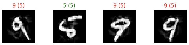
Flag ML 108.2: Smaller Perturbation (10 pts)
Make these changes:The modified images have different patterns of blurry smudges added, as shown below.
- Change the maximum perturbation to 2.0
- Change the maximum iterations to 50
As in flag 108.1, find all the correct predictions in the 25 images in the bottom row and concatenate their values to form the flag.
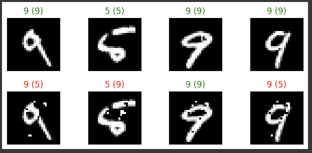
Flag ML 108.3: Different Perturbation Type (10 pts)
Make these changes:The modified images now have only bright or dark pixels added, rather than grays, as shown below.
- Change the perturbation type to l1 (the letter l followed by the digit 1)
- Change the maximum perturbation to 12.0
- Change the maximum iterations to 40
As in flag 108.1, find all the correct predictions in the 25 images in the bottom row and concatenate their values to form the flag.
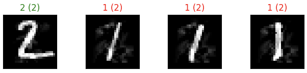
Flag ML 108.4: Different Digits (10 pts)
Make these changes:The first four modified images are shown below.
- Use 200 training samples
- Use 400 validation and test set samples
- Use the digits 1 and 2
- Use the perturbation type l2 (the letter l followed by the digit 2)
- Use maximum perturbation 2.1
- Set the maximum iterations to 40
As in flag 108.1, find all the correct predictions in the 25 images in the bottom row and concatenate their values to form the flag.
Posted and video added 5-3-23
Perturbation type in flags 3 and 4 fixed 12-13-23
Image for "An Evasion Attack" updated 7-23-24
Jupyter note added 5-15-25