Hands-On Machine Learning with Scikit-Learn, Keras, and TensorFlow 3rd Edition, by Aurélien Géron
https://colab.research.google.com/If you see a blue "Sign In" button at the top right, click it and log into a Google account.
From the menu, click File, "New notebook".
from sklearn.datasets import fetch_openml

mnist = fetch_openml('mnist_784', as_frame=False, parser="auto")
print(mnist.DESCR)
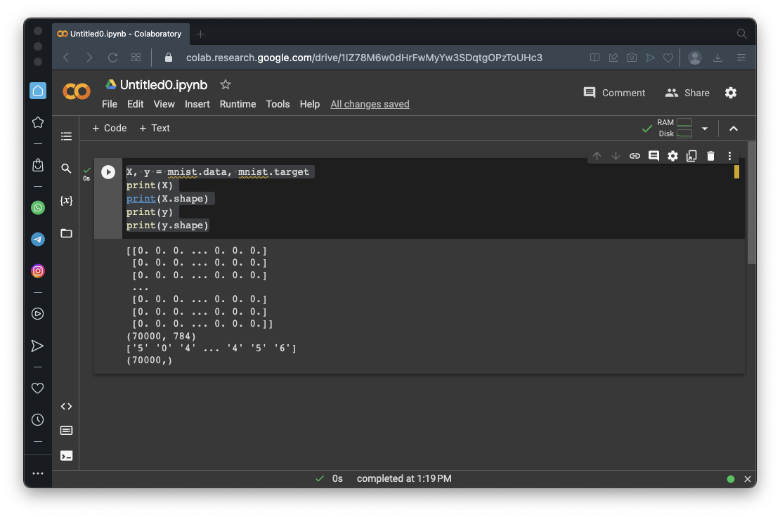
X, y = mnist.data, mnist.target
print(X)
print(X.shape)
print(y)
print(y.shape)
y contains the number that was written, for all 70000 images. Notice that the first two images are '5'and '0'.
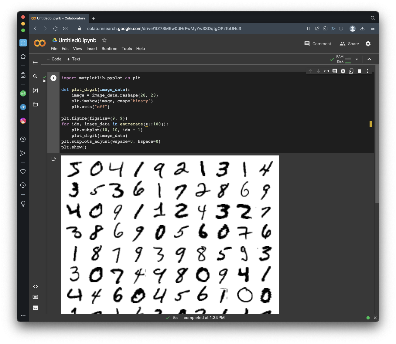
import matplotlib.pyplot as plt

def plot_digit(image_data):
    image = image_data.reshape(28, 28)
    plt.imshow(image, cmap="binary")
    plt.axis("off")

plt.figure(figsize=(9, 9))
for idx, image_data in enumerate(X[:100]):
    plt.subplot(10, 10, idx + 1)
    plot_digit(image_data)
plt.subplots_adjust(wspace=0, hspace=0)
plt.show()
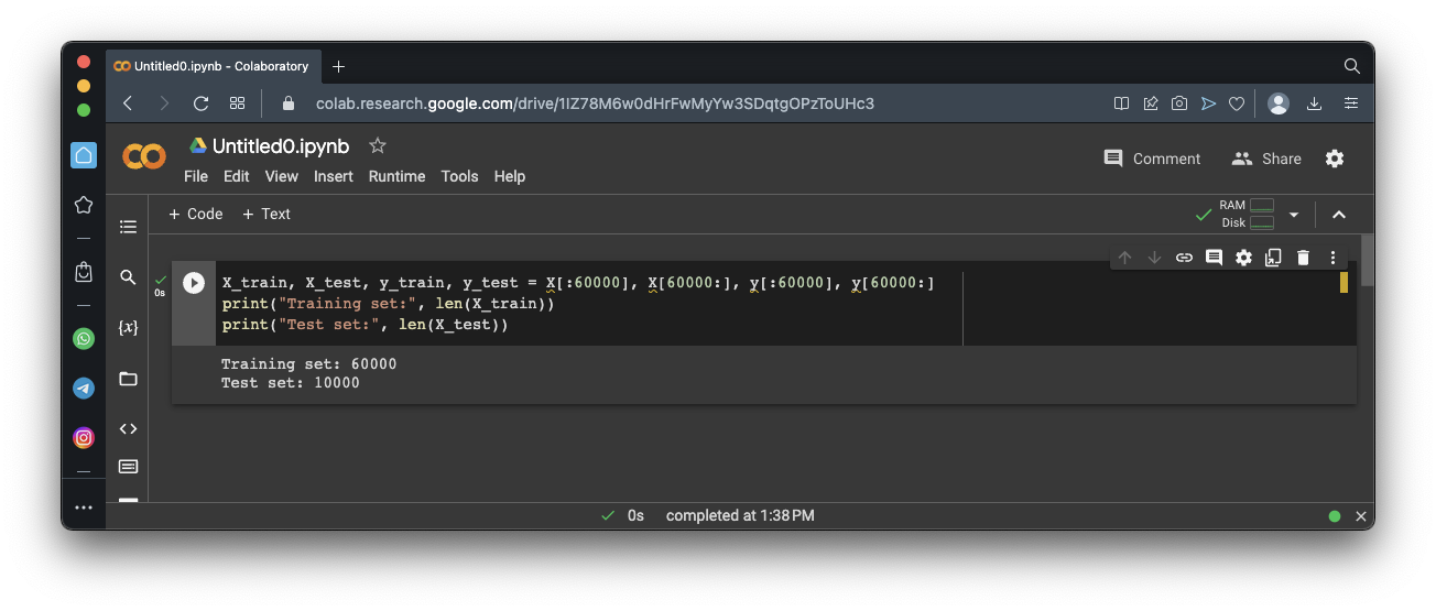
X_train, X_test, y_train, y_test = X[:60000], X[60000:], y[:60000], y[60000:]
print("Training set:", len(X_train))
print("Test set:", len(X_test))
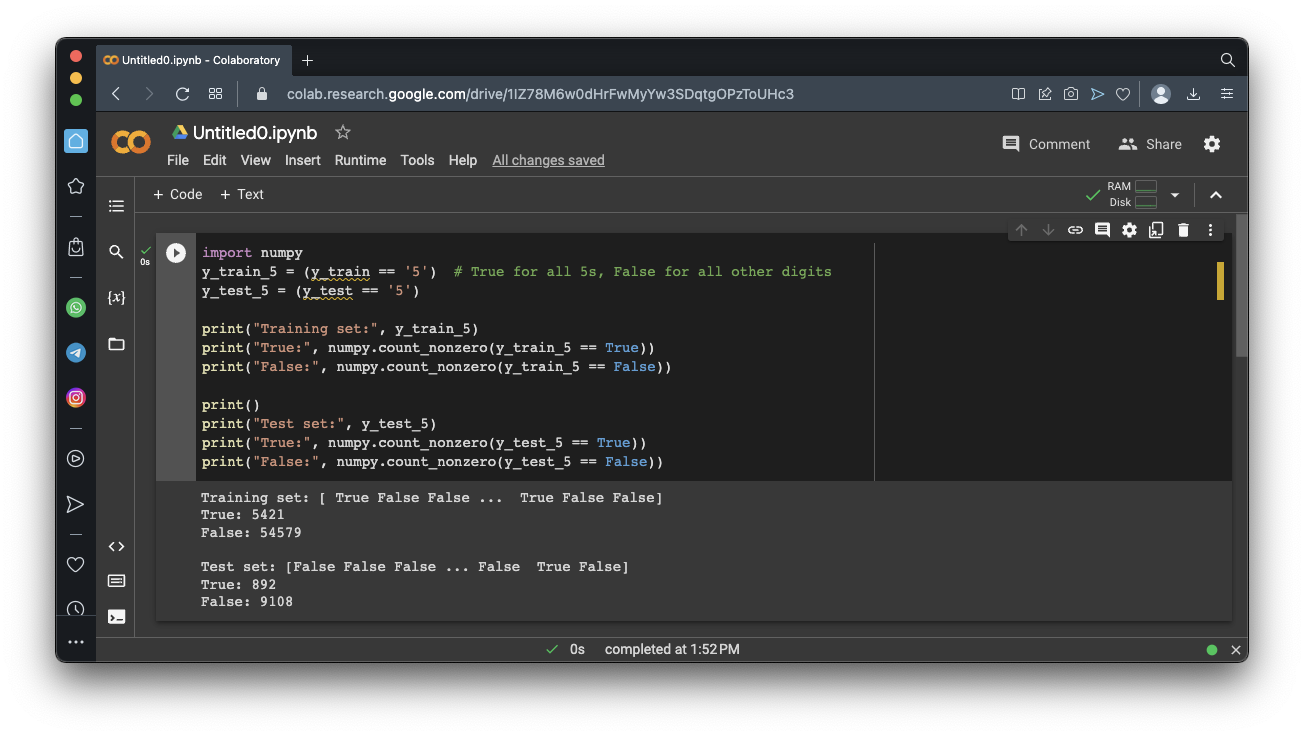
import numpy
y_train_5 = (y_train == '5')  # True for all 5s, False for all other digits
y_test_5 = (y_test == '5')

print("Training set:", y_train_5)
print("True:", numpy.count_nonzero(y_train_5 == True))
print("False:", numpy.count_nonzero(y_train_5 == False))

print()
print("Test set:", y_test_5)
print("True:", numpy.count_nonzero(y_test_5 == True))
print("False:", numpy.count_nonzero(y_test_5 == False))
The learning is a process of choosing the weights.
from sklearn.linear_model import SGDClassifier
sgd_clf = SGDClassifier(random_state=42, verbose=2)
sgd_clf.fit(X_train, y_train_5)
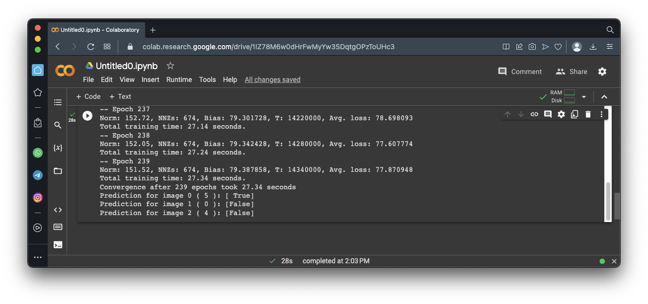
print("Prediction for image 0 (",y[0],"):", sgd_clf.predict([X[0]]))
print("Prediction for image 1 (",y[1],"):", sgd_clf.predict([X[1]]))
print("Prediction for image 2 (",y[2],"):", sgd_clf.predict([X[2]]))
Execute these commands to perform cross-validation on our model:
from sklearn.model_selection import cross_val_score
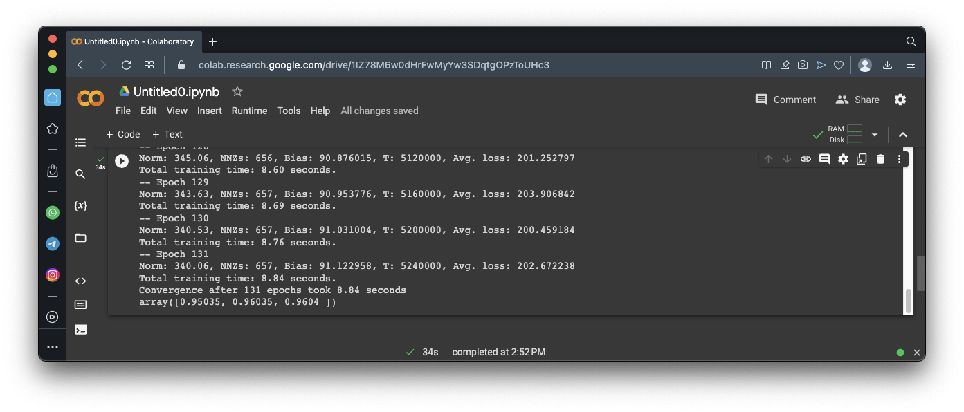
cross_val_score(sgd_clf, X_train, y_train_5, cv=3, scoring="accuracy")
However, remember that our data set is 90% 'False' values, so that is not as good as it sounds.
The cross_val_predict() function will perform 3-fold cross validation, and return the predicted values.
The confusion_matrix() function counts the hits and misses.
from sklearn.model_selection import cross_val_predict
y_train_pred = cross_val_predict(sgd_clf, X_train, y_train_5, cv=3)
from sklearn.metrics import confusion_matrix
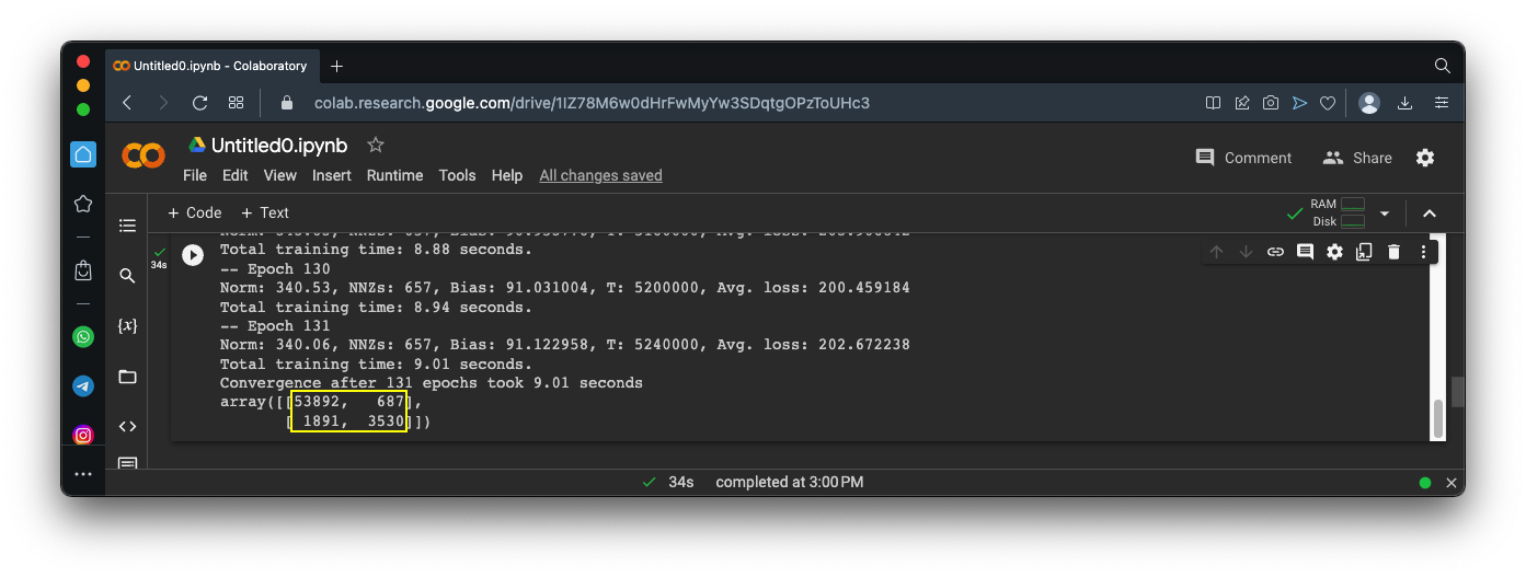
cm = confusion_matrix(y_train_5, y_train_pred)
cm
The first row contains most of the images--these are the non-5 images. The model incorrectly called 687 of them 5's.
The second row is the fives. The model incorrectly called 1891 of them non-5.
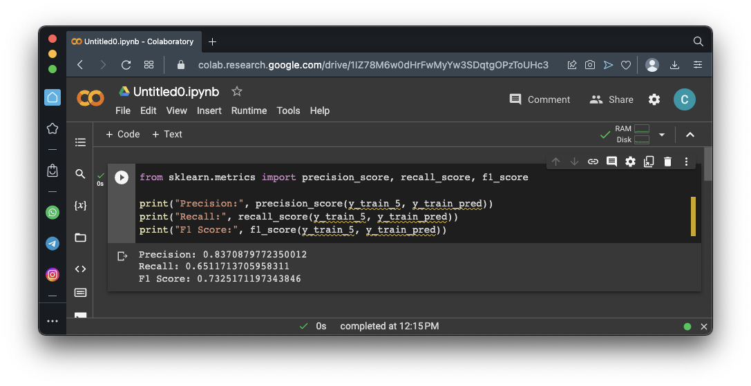
Precision = (True Positives) / (True Positives + False Positives)From the matrix in the image above:
Precision = 3530 / (3530 + 687) = 0.837 = 83.7%Precision alone is not a good measure of quality, because we could make a model that is very picky, only identifying perfect matches as positive.
This model would have no False Positives, and therefore a Precision of 100%, but it would have many False Negatives.
So a second measure is needed: Recall.
Here's the formula for Recall:
Recall = (True Positives) / (True Positives + False Negatives)From the matrix in the image above:
Recall = 3530 / (3530 + 1891) = 0.651 = 65.1%
F1 = 2 x (Precision x Recall) / (Precision + Recall)The F1 score will only be near 1 if both Precision and Recall are. From the values above:
F1 = 2 x (0.837 x 0.651) / (0.837 + 0.651) = 0.732 = 73.2%
from sklearn.metrics import precision_score, recall_score, f1_score

print("Precision:", precision_score(y_train_5, y_train_pred))
print("Recall:", recall_score(y_train_5, y_train_pred))
print("F1 Score:", f1_score(y_train_5, y_train_pred))
But suppose you want asymmetric results--consider a facial recognition scanner to detect known thieves in a retail store. You really want to avoid False Positives, which accuse innocent shoppers of being thieves. It's worth accepting a higher False Negative rate to achieve that end.
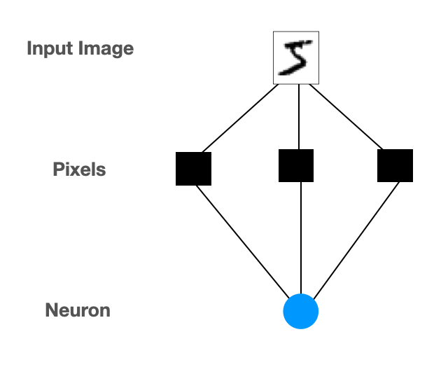
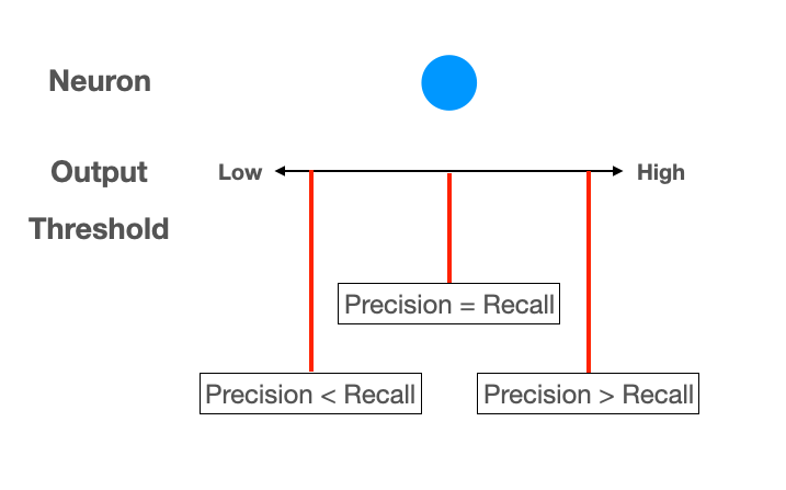
Consider the situation shown below.
The neuron has an output signal level. Values above the threshold are classified as 5's, values below that level are classified as non-5's.
If the threshold is low, many outputs are classified as 5's, producing many False Positives. This makes Precision low.
If the threshold is high, many outputs are classified as non-5's, producing many False Negatives. This makes Recall low.
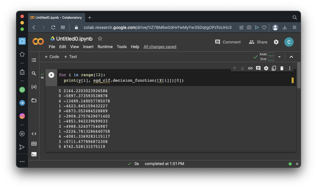
for i in range(12):
  print(y[i], sgd_clf.decision_function([X[i]])[0])
By default, sklearn uses a threshold of zero.
If the threshold were 3000, the first image would be classified as non-5, but the last one would still be classified as 5.
y_scores = cross_val_predict(sgd_clf, X_train, y_train_5, cv=3,
                             method="decision_function")
from sklearn.metrics import precision_recall_curve
precisions, recalls, thresholds = precision_recall_curve(y_train_5, y_scores)

import matplotlib.pyplot as plt
plt.plot(thresholds, precisions[:-1], "b--", label="Precision", linewidth=2)
plt.plot(thresholds, recalls[:-1], "g-", label="Recall", linewidth=2)
plt.grid()
plt.axis([-50000, 50000, 0, 1])
plt.xlabel("Threshold")
plt.legend(loc="center right")
plt.show()
Precision gets noisy at high thresholds, where there are very few positives.
Flag ML 105.1: Precision for Threshold 3000 (15 pts)
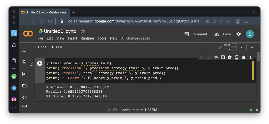
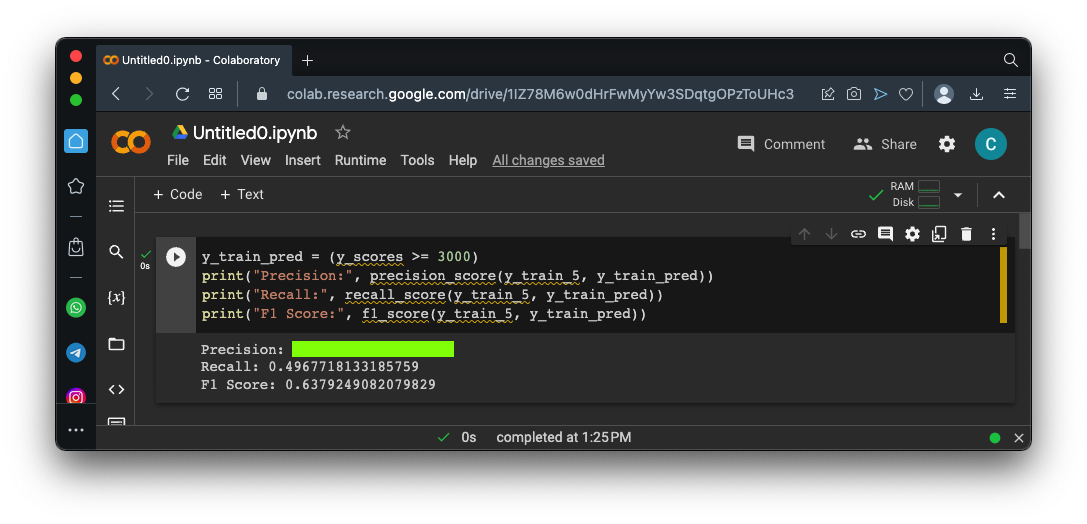
Execute these commands to calculate the Precision and Recall for a threshold of 0:As shown below, you get the same values we saw above, because the default threshold is zero.y_train_pred = (y_scores >= 0) print("Precision:", precision_score(y_train_5, y_train_pred)) print("Recall:", recall_score(y_train_5, y_train_pred)) print("F1 Score:", f1_score(y_train_5, y_train_pred))Change the zero in the first line to 3000 and calculate the values again. The flag is the precision value, covered by a green rectangle in the image below.
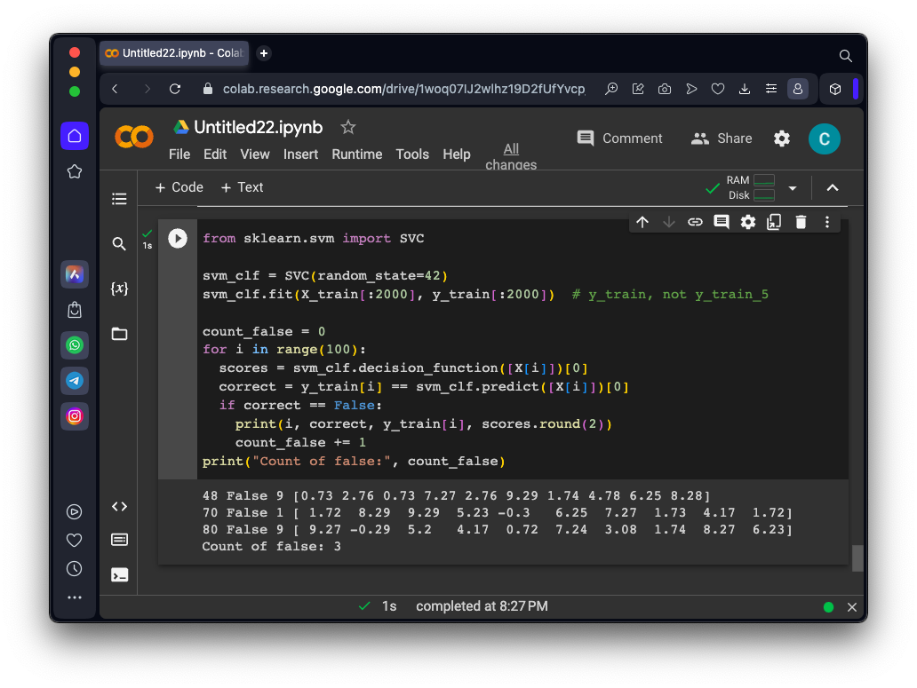
from sklearn.svm import SVC

svm_clf = SVC(random_state=42)
svm_clf.fit(X_train[:2000], y_train[:2000])  # y_train, not y_train_5

count_false = 0
for i in range(100):
  scores = svm_clf.decision_function([X[i]])[0]
  correct = y_train[i] == svm_clf.predict([X[i]])[0]
  if correct == False:
    print(i, correct, y_train[i], scores.round(2))
    count_false += 1
print("Count of false:", count_false)
As shown below, it was wrong only 3 times, and one of those errors was image 80. Image 80 was actually a "9", but was classified as a "0" because the decision function for "0" was 9.27, the largest value on that line.
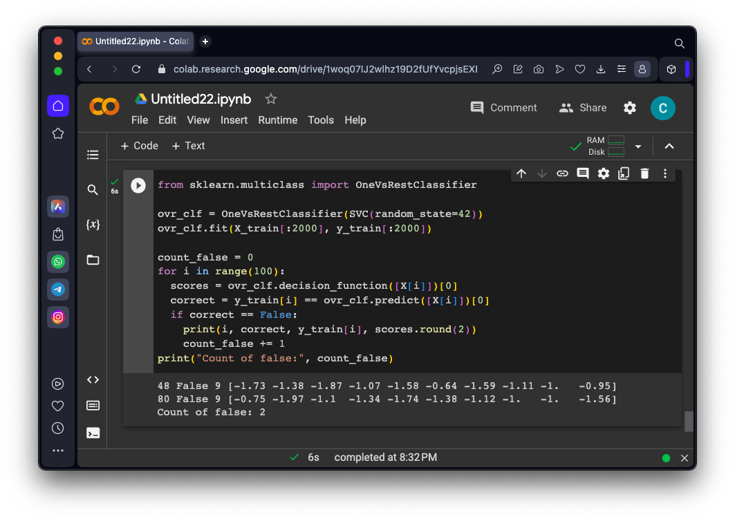
from sklearn.multiclass import OneVsRestClassifier

ovr_clf = OneVsRestClassifier(SVC(random_state=42))
ovr_clf.fit(X_train[:2000], y_train[:2000])

count_false = 0
for i in range(100):
  scores = ovr_clf.decision_function([X[i]])[0]
  correct = y_train[i] == ovr_clf.predict([X[i]])[0]
  if correct == False:
    print(i, correct, y_train[i], scores.round(2))
    count_false += 1
print("Count of false:", count_false)
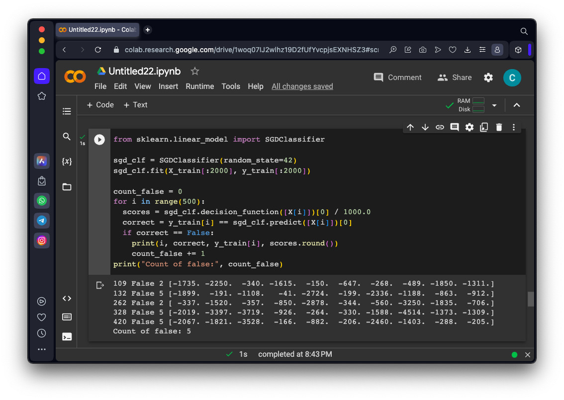
from sklearn.linear_model import SGDClassifier

sgd_clf = SGDClassifier(random_state=42)
sgd_clf.fit(X_train[:2000], y_train[:2000])

count_false = 0
for i in range(500):
  scores = sgd_clf.decision_function([X[i]])[0] / 1000.0
  correct = y_train[i] == sgd_clf.predict([X[i]])[0]
  if correct == False:
    print(i, correct, y_train[i], scores.round())
    count_false += 1
print("Count of false:", count_false)
As shown below, this model is much better, making only 5 errors in the first 500 training images!
Execute these commands to examine its performance on the test set:
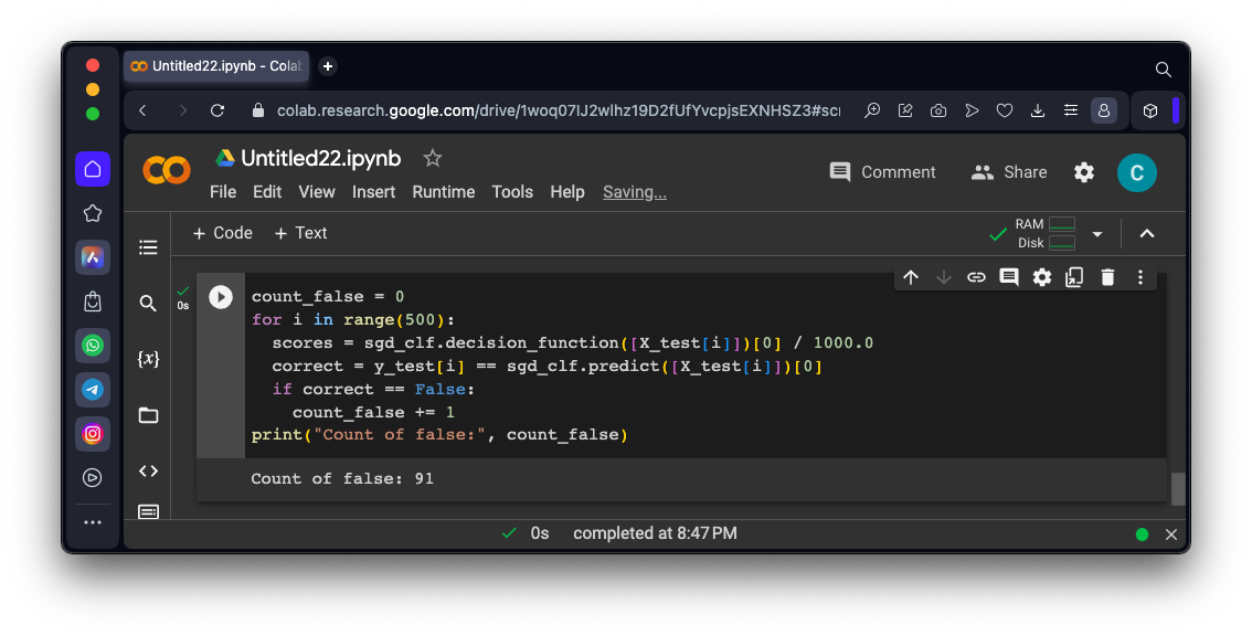
count_false = 0
for i in range(500):
  scores = sgd_clf.decision_function([X_test[i]])[0] / 1000.0
  correct = y_test[i] == sgd_clf.predict([X_test[i]])[0]
  if correct == False:
    count_false += 1
print("Count of false:", count_false)
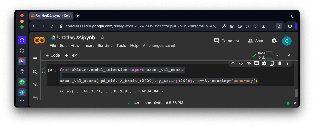
from sklearn.model_selection import cross_val_score

cross_val_score(sgd_clf, X_train[:2000], y_train[:2000], cv=3, scoring="accuracy")
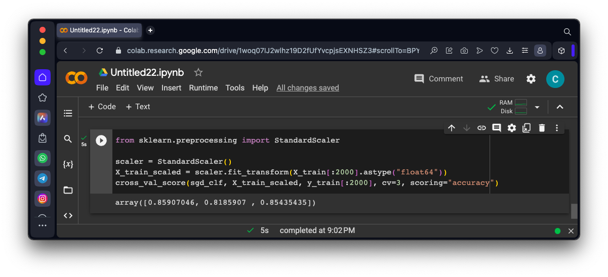
from sklearn.preprocessing import StandardScaler

scaler = StandardScaler()
X_train_scaled = scaler.fit_transform(X_train[:2000].astype("float64"))
cross_val_score(sgd_clf, X_train_scaled, y_train[:2000], cv=3, scoring="accuracy")
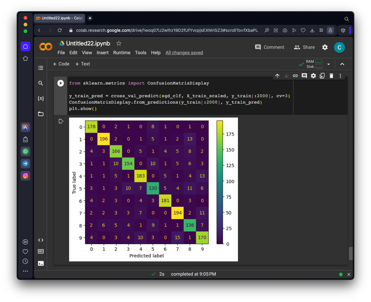
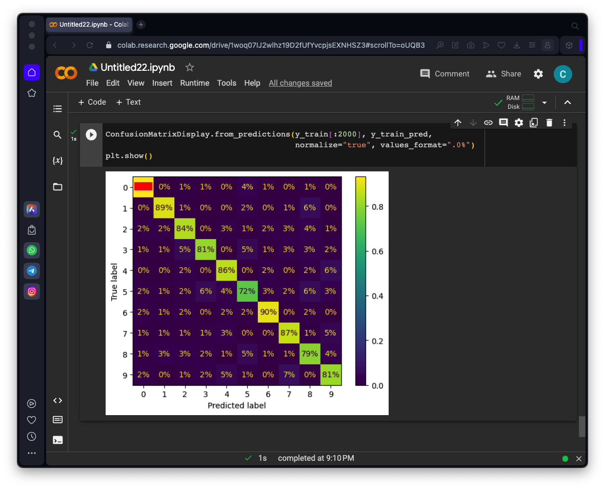
from sklearn.metrics import ConfusionMatrixDisplay

y_train_pred = cross_val_predict(sgd_clf, X_train_scaled, y_train[:2000], cv=3)
ConfusionMatrixDisplay.from_predictions(y_train[:2000], y_train_pred)
plt.show()
ConfusionMatrixDisplay.from_predictions(y_train[:2000], y_train_pred,
                                        normalize="true", values_format=".0%")
plt.show()
Flag ML 105.2: Correct Percentage for 0's (10 pts)
The flag is covered by a red rectangle in the image below.
Posted and video added 4-20-23
parser="auto" added to fetch_openml() call 4-26-23
Minor typo fixed 5-3-23
Video updated 5-3-23
Typo fixed 9-8-23
Another minor text error fixed 7-23-24