Hands-On Machine Learning with Scikit-Learn, Keras, and TensorFlow 3rd Edition, by Aurélien Géron
https://colab.research.google.com/If you see a blue "Sign In" button at the top right, click it and log into a Google account.
From the menu, click File, "New notebook".
import sys
assert sys.version_info >= (3, 7)
from packaging import version
import sklearn
assert version.parse(sklearn.__version__) >= version.parse("1.0.1")
from pathlib import Path
import pandas as pd
import tarfile
import urllib.request
def load_housing_data():
tarball_path = Path("datasets/housing.tgz")
if not tarball_path.is_file():
Path("datasets").mkdir(parents=True, exist_ok=True)
url = "https://github.com/ageron/data/raw/main/housing.tgz"
urllib.request.urlretrieve(url, tarball_path)
with tarfile.open(tarball_path) as housing_tarball:
housing_tarball.extractall(path="datasets")
return pd.read_csv(Path("datasets/housing/housing.csv"))
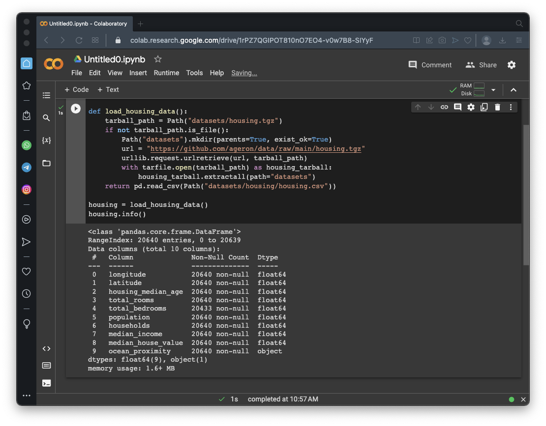
housing = load_housing_data()
housing.info()
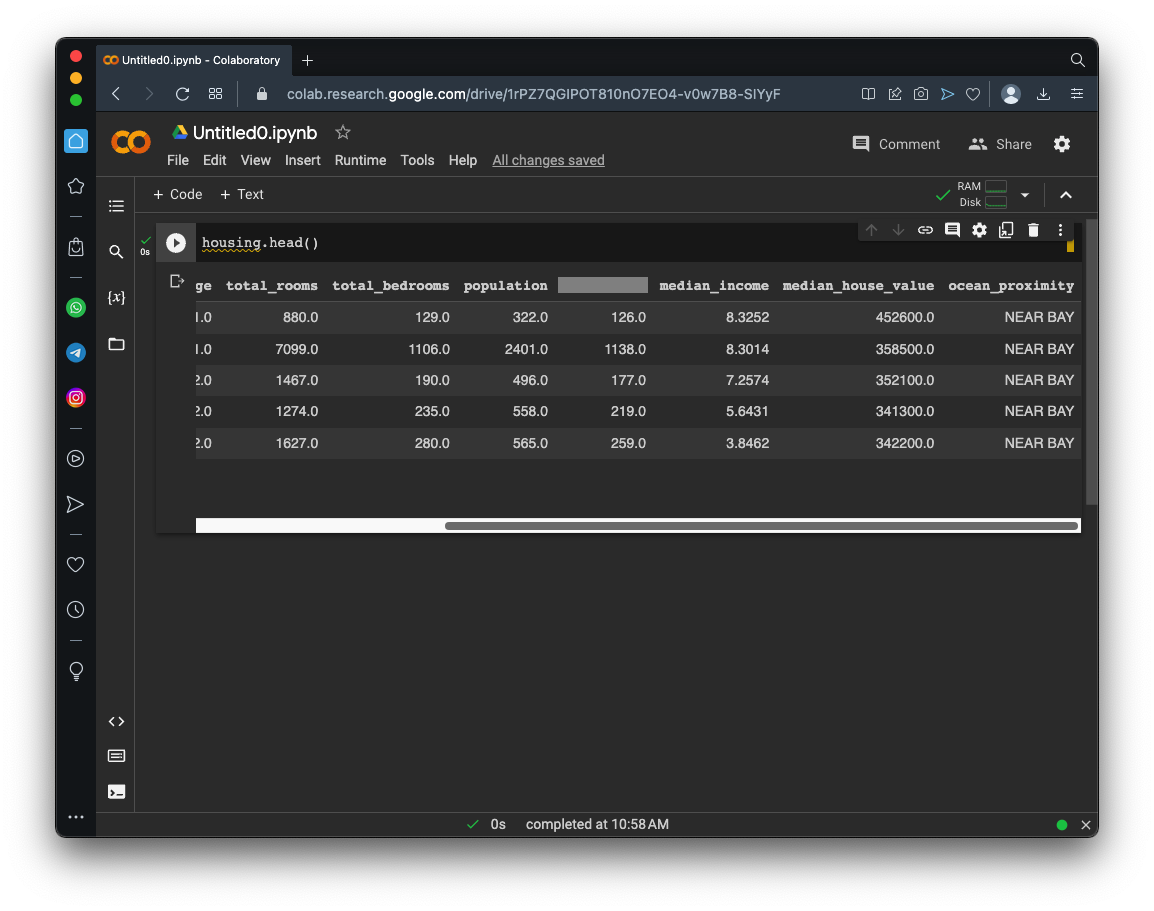
housing.head()
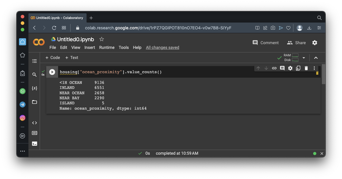
housing["ocean_proximity"].value_counts()
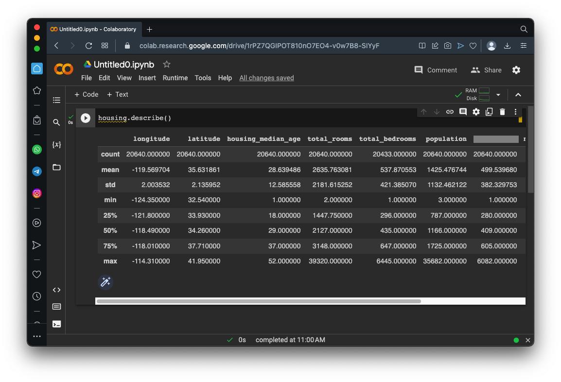
housing.describe()
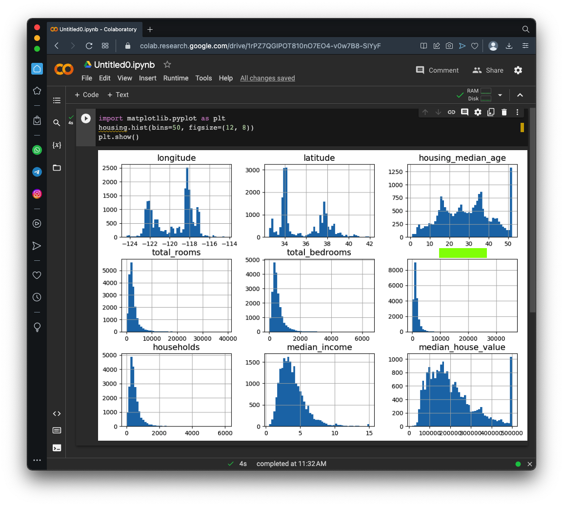
Flag ML 104.1: Histograms (5 pts)
Execute these commands to see histogram plots of each numerical attribute:As shown below, the plots make it easy to see the distributions of the data.The flag is covered by a green rectangle in the image below.
import numpy as np

def shuffle_and_split_data(data, test_ratio):
    shuffled_indices = np.random.permutation(len(data))
    test_set_size = int(len(data) * test_ratio)
    test_indices = shuffled_indices[:test_set_size]
    train_indices = shuffled_indices[test_set_size:]
    return data.iloc[train_indices], data.iloc[test_indices]

train_set, test_set = shuffle_and_split_data(housing, 0.2)
print("Training set:", len(train_set))
print("Test set:", len(test_set))
print("Head of test set:")
print(test_set.head())
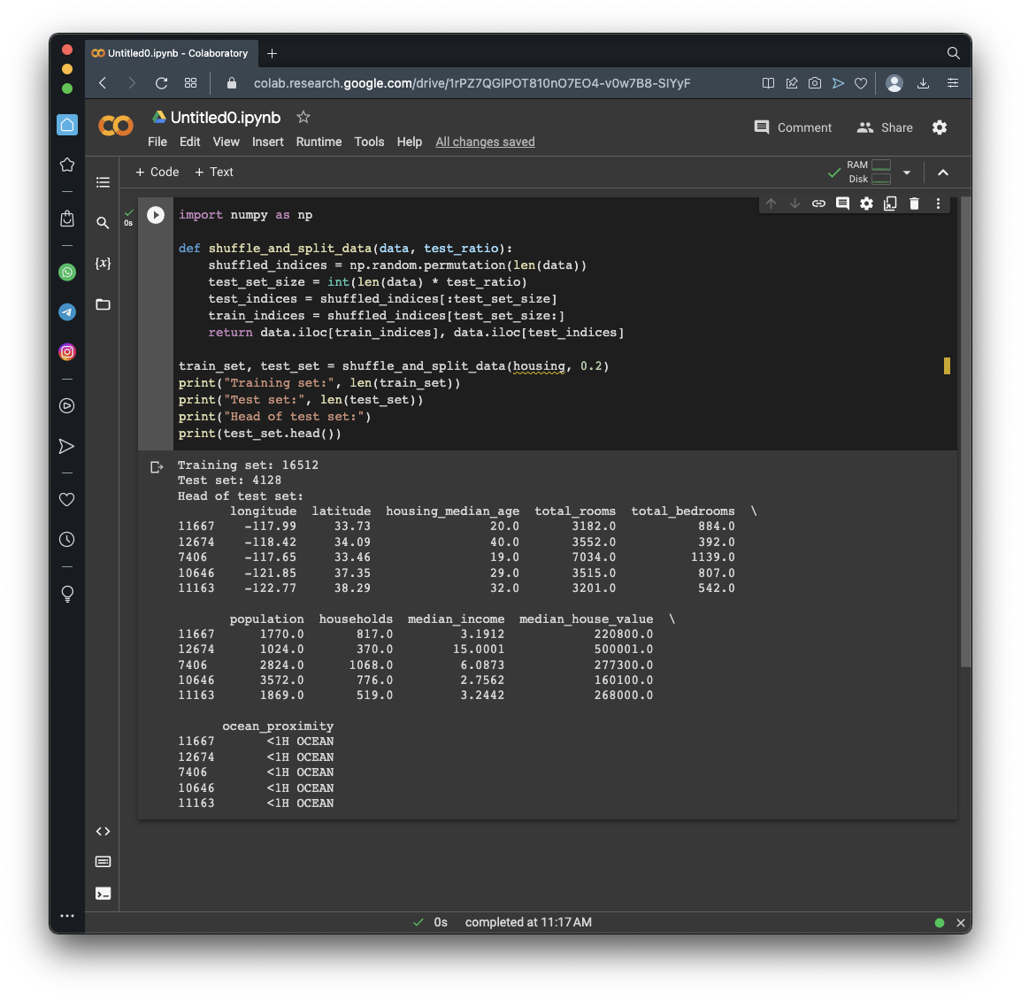
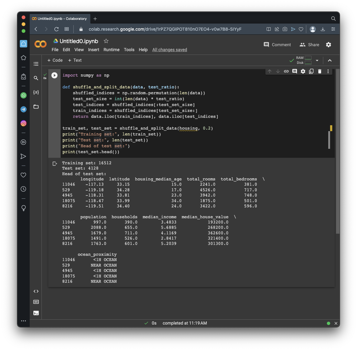
Run the previous commands again.
As shown below, different rows are selected each time. This is not the best way to select a training set, because if you run the model many times, the training will see all the data, which is what you want to avoid.
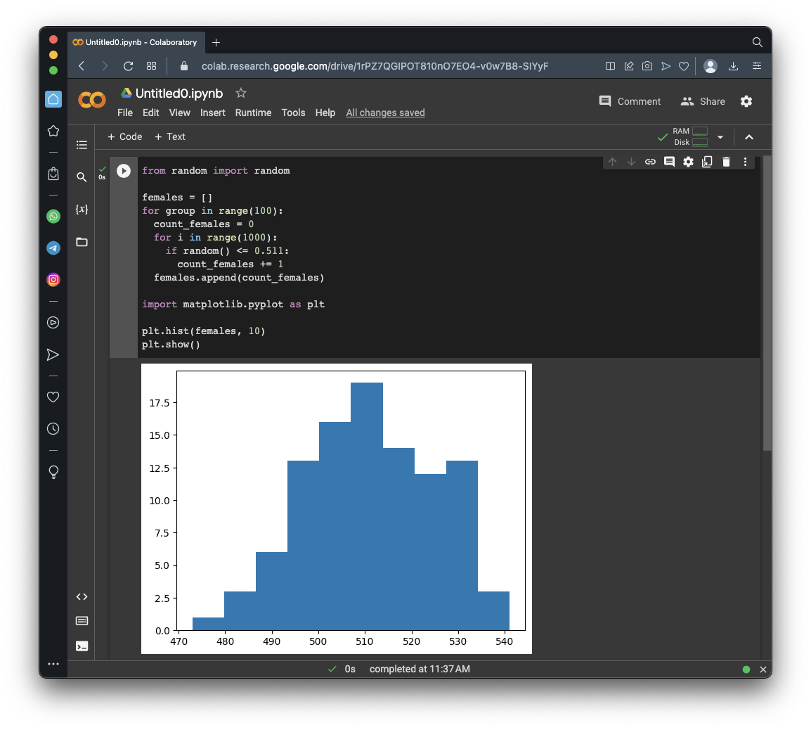
Execute these commands to create 100 random samples of 1000 people and gather the percentage of females in each sample:
from random import random

females = []
for group in range(100):
  count_females = 0
  for i in range(1000):
    if random() <= 0.511:
      count_females += 1
  females.append(count_females)

import matplotlib.pyplot as plt

plt.hist(females, 10)
plt.show()
In this case, we are training a model to predict a house price in California. We'll postulate that median income is very important to predict house prices, so we want to correctly represent the categories of median income.
As you saw above, in the "Flag ML 104.1: Histograms" section, median income is mostly between 1.5 and 6, but there are some values up to 15.
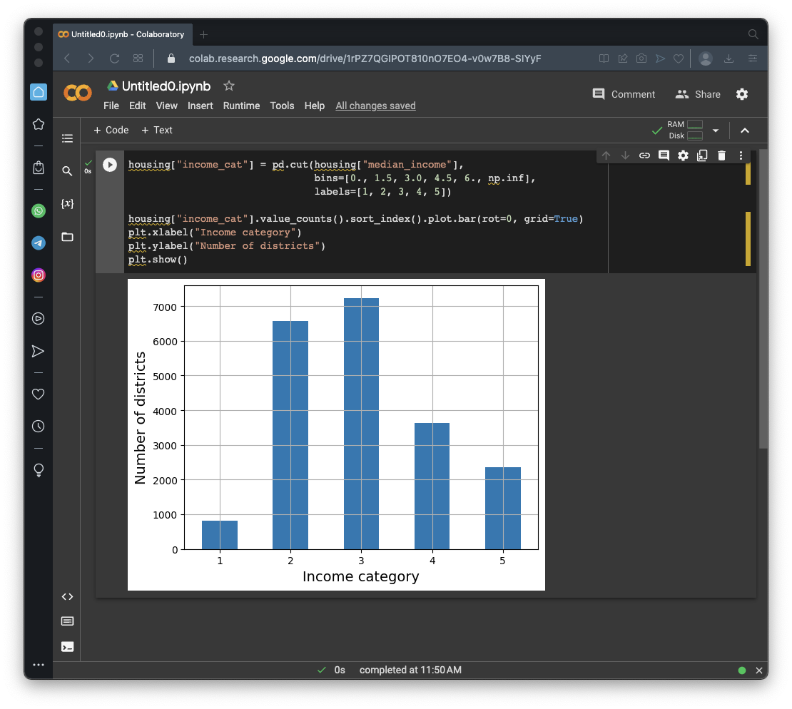
We'll use these five categories:
housing["income_cat"] = pd.cut(housing["median_income"],
                               bins=[0., 1.5, 3.0, 4.5, 6., np.inf],
                               labels=[1, 2, 3, 4, 5])

housing["income_cat"].value_counts().sort_index().plot.bar(rot=0, grid=True)
plt.xlabel("Income category")
plt.ylabel("Number of districts")
plt.show()
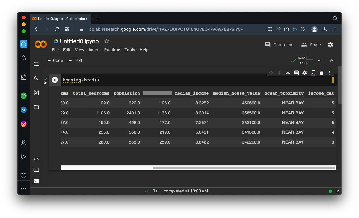
housing.head()
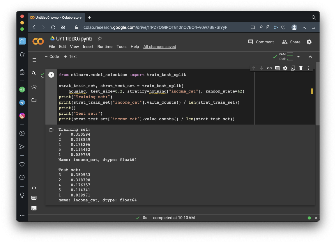
from sklearn.model_selection import train_test_split

strat_train_set, strat_test_set = train_test_split(
    housing, test_size=0.2, stratify=housing["income_cat"], random_state=42)
print("Training set:")
print(strat_train_set["income_cat"].value_counts() / len(strat_train_set))
print()
print("Test set:")
print(strat_test_set["income_cat"].value_counts() / len(strat_test_set))
import numpy as np

def shuffle_and_split_data(data, test_ratio):
    shuffled_indices = np.random.permutation(len(data))
    test_set_size = int(len(data) * test_ratio)
    test_indices = shuffled_indices[:test_set_size]
    train_indices = shuffled_indices[test_set_size:]
    return data.iloc[train_indices], data.iloc[test_indices]

train_set, test_set = shuffle_and_split_data(housing, 0.2)
print("Training set:", len(train_set))
print("Test set:", len(test_set))
print("Head of test set:")
print(test_set.head())
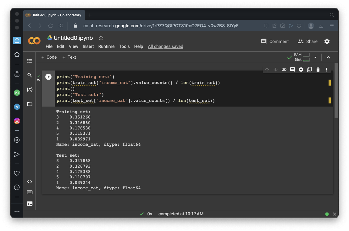
print("Training set:")
print(train_set["income_cat"].value_counts() / len(train_set))
print()
print("Test set:")
print(test_set["income_cat"].value_counts() / len(test_set))
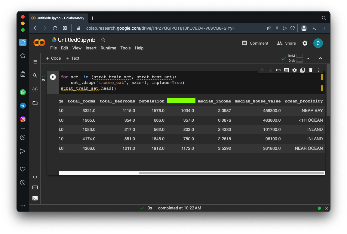
Flag ML 104.2 Removing the "income_cat" column (10 pts)
Execute these commands to remove the income_cat column and see the first five rows to verify that it's gone:As shown below, the income_cat column is gone.for set_ in (strat_train_set, strat_test_set): set_.drop("income_cat", axis=1, inplace=True) strat_train_set.head()The flag is covered by a green rectangle in the image below.
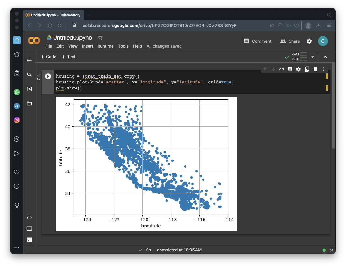
housing = strat_train_set.copy()
housing.plot(kind="scatter", x="longitude", y="latitude", grid=True)
plt.show()
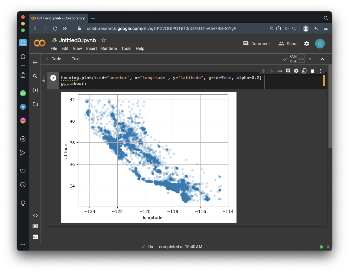
housing.plot(kind="scatter", x="longitude", y="latitude", grid=True, alpha=0.2)
plt.show()
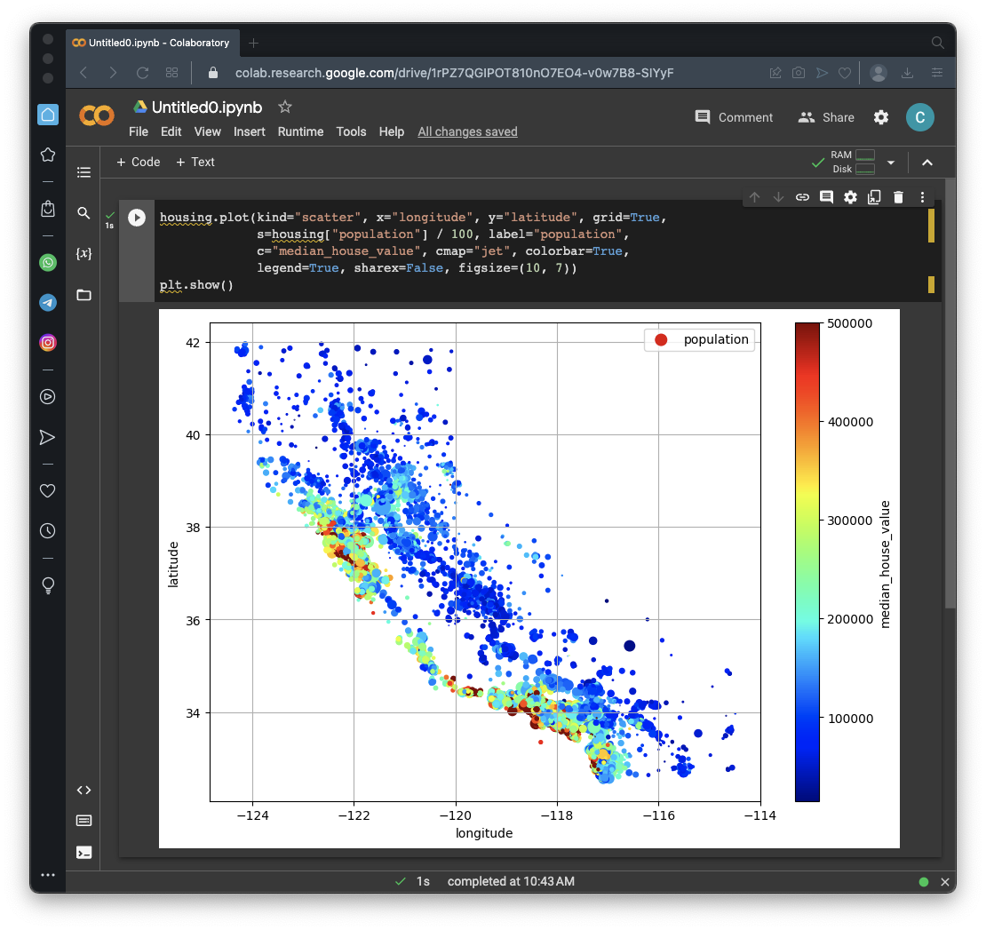
housing.plot(kind="scatter", x="longitude", y="latitude", grid=True,
             s=housing["population"] / 100, label="population",
             c="median_house_value", cmap="jet", colorbar=True,
             legend=True, sharex=False, figsize=(10, 7))
plt.show()
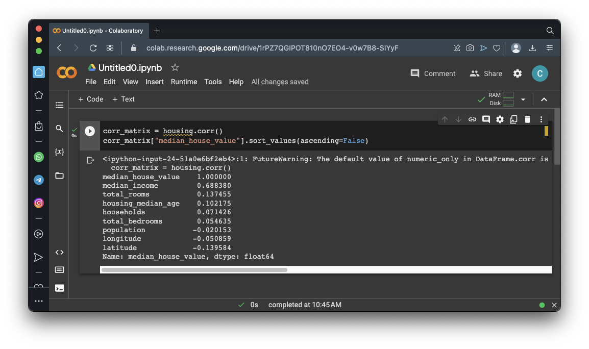
corr_matrix = housing.corr(numeric_only=True)
corr_matrix["median_house_value"].sort_values(ascending=False)
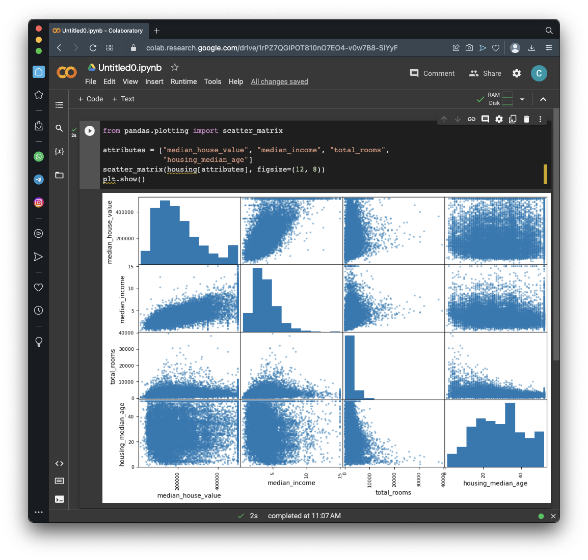
from pandas.plotting import scatter_matrix

attributes = ["median_house_value", "median_income", "total_rooms",
              "housing_median_age"]
scatter_matrix(housing[attributes], figsize=(12, 8))
plt.show()
The leftmost plot is a histogram of median_house_value, which we've seen before, and it's not helpful here.
The remaining three plots show how much the other parameters influence median_house_value, and make it obvious that median_income has a large effect, and the other two parameters have very little effect.
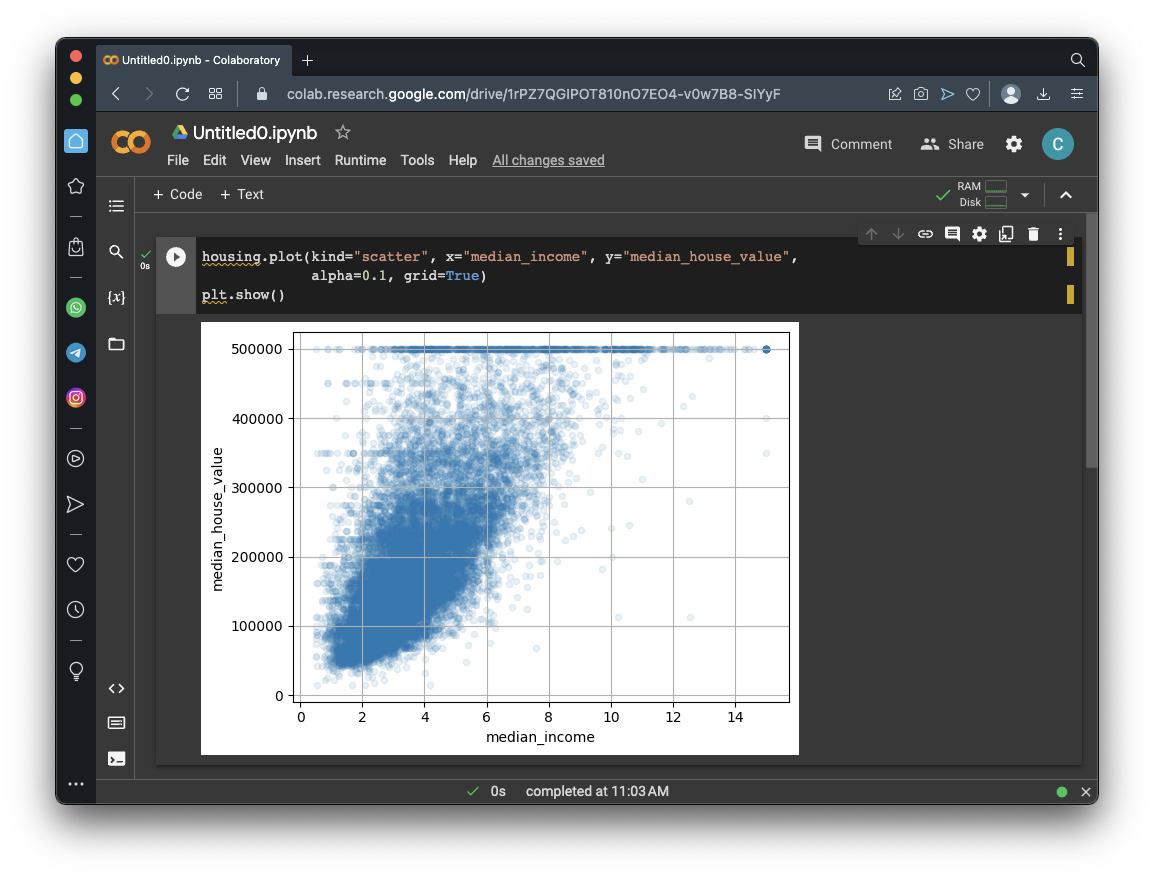
Execute these commands to see the scatter plot of median_income and median_house_value in more detail:
housing.plot(kind="scatter", x="median_income", y="median_house_value",
             alpha=0.1, grid=True)
plt.show()
It might be best to remove the districts on those lines from the data to prevent the model from learning to reproduce those artifacts which don't represent accurate inputs.
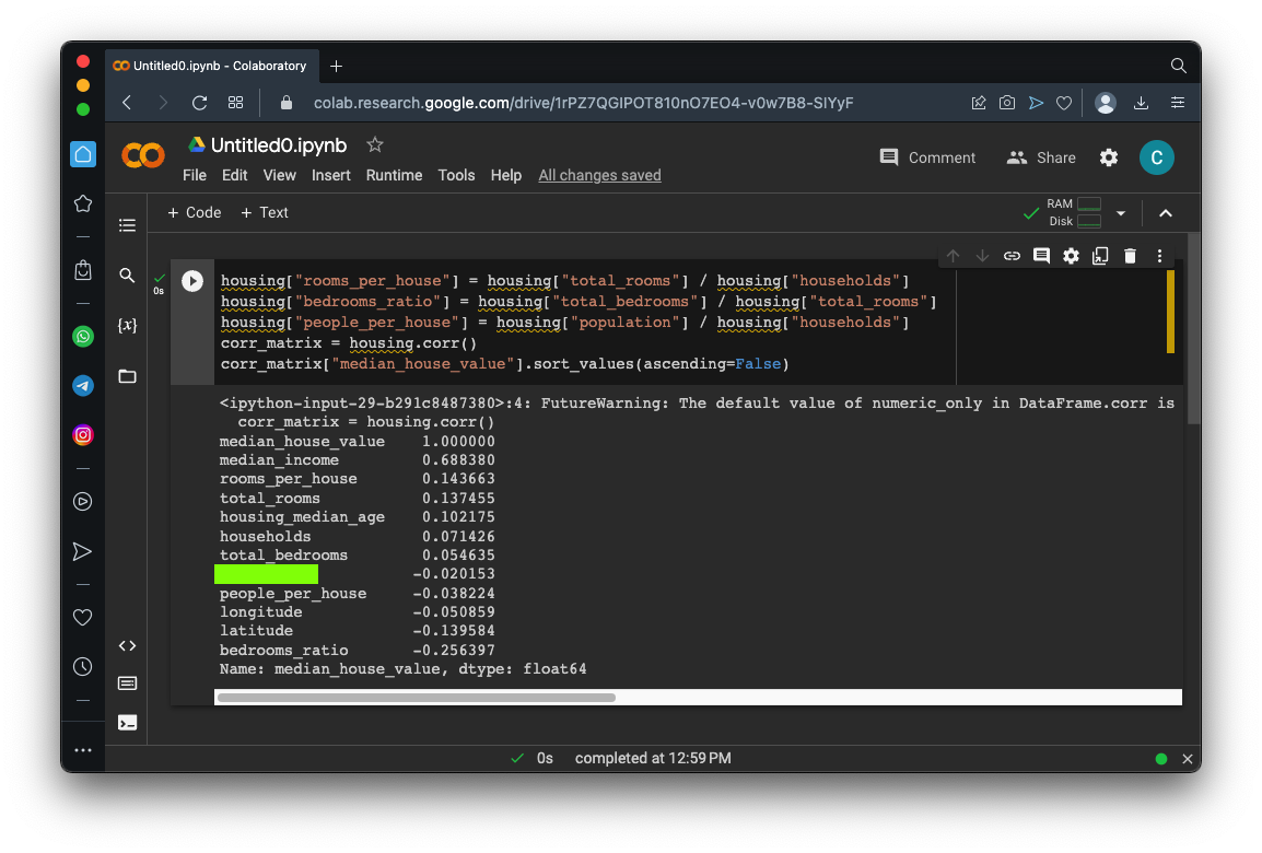
Flag ML 104.3: Attribute Combinations (5 pts)
Execute these commands to create three new columns combining attributes, and calculate the correlations:As shown below, bedrooms_ratio has a strong negative correlation of -0.25, much larger than the correlations of total_bedrooms or total_rooms.The flag is covered by a green rectangle in the image below.
Posted 4-13-23
Video added 4-20-23
Video updated 5-3-23
Several code updates 6-28-24