Deblur Images using Autoencoders 82% Acc
https://colab.research.google.com/If you see a blue "Sign In" button at the top right, click it and log into a Google account.
From the menu, click File, "New notebook".
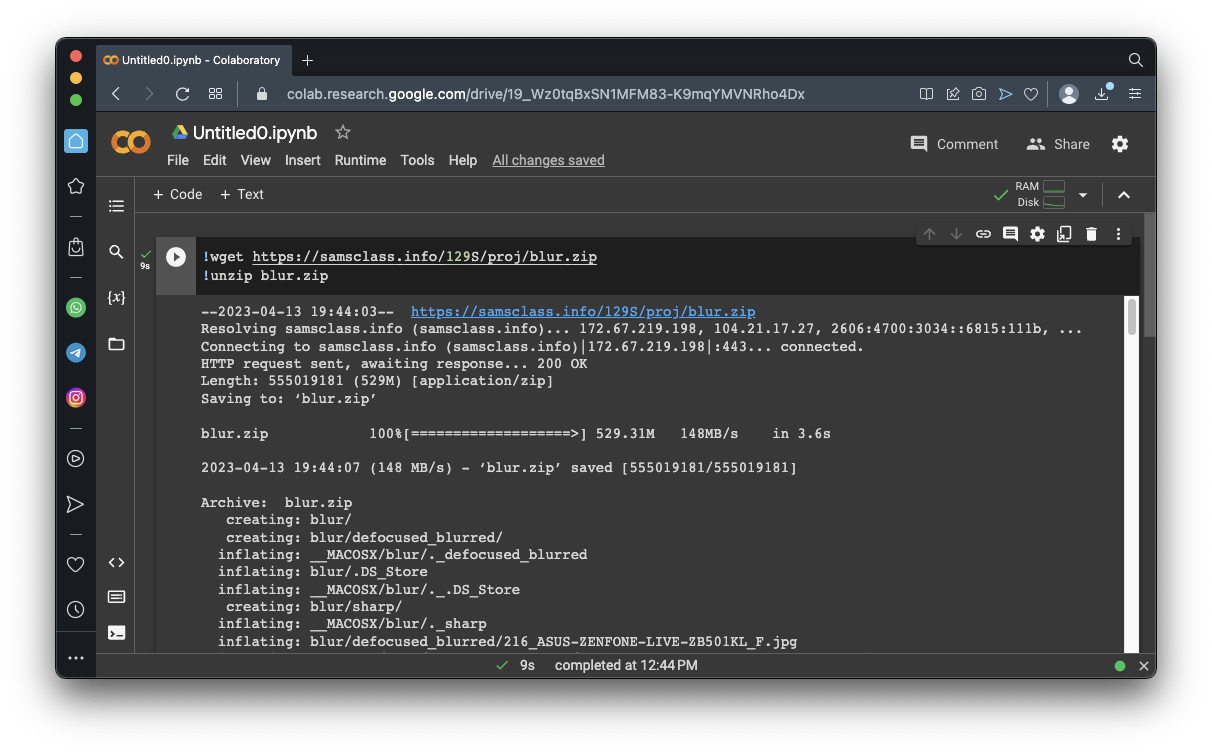
!wget https://samsclass.info/129S/proj/blur.zip
!unzip blur.zip
import numpy as np
import pandas as pd
import matplotlib.pyplot as plt

%matplotlib inline
import random
import cv2
import os
import tensorflow as tf
from tqdm import tqdm

seed = 21
random.seed(seed)
np.random.seed(seed)

good_frames = 'blur/sharp'
bad_frames = 'blur/defocused_blurred'

clean_frames = []
for file in tqdm(sorted(os.listdir(good_frames))):
    if any(extension in file for extension in ['.jpg', 'jpeg', '.png']):
        image = tf.keras.preprocessing.image.load_img(good_frames + '/' + file, target_size=(128,128))
        image = tf.keras.preprocessing.image.img_to_array(image).astype('float32') / 255
        clean_frames.append(image)

clean_frames = np.array(clean_frames)
blurry_frames = []
for file in tqdm(sorted(os.listdir(bad_frames))):
    if any(extension in file for extension in ['.jpg', 'jpeg', '.png']):
        image = tf.keras.preprocessing.image.load_img(bad_frames + '/' + file, target_size=(128,128))
        image = tf.keras.preprocessing.image.img_to_array(image).astype('float32') / 255
        blurry_frames.append(image)

blurry_frames = np.array(blurry_frames)

r = random.randint(0, len(clean_frames)-1)
print(r)
fig = plt.figure()
fig.subplots_adjust(hspace=0.1, wspace=0.2)
ax = fig.add_subplot(1, 2, 1)
ax.imshow(clean_frames[r])
ax = fig.add_subplot(1, 2, 2)
ax.imshow(blurry_frames[r])
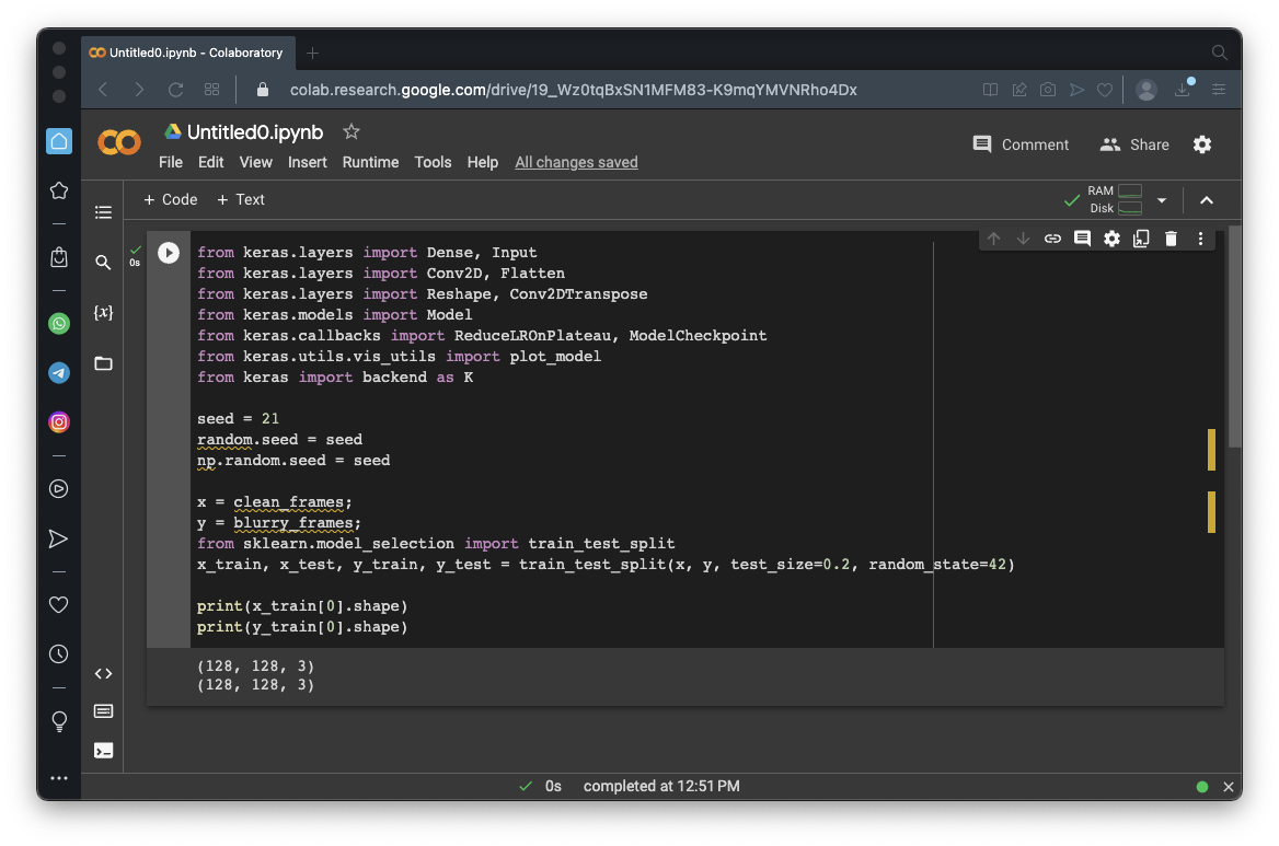
from keras.layers import Dense, Input
from keras.layers import Conv2D, Flatten
from keras.layers import Reshape, Conv2DTranspose
from keras.models import Model
from keras.callbacks import ReduceLROnPlateau, ModelCheckpoint
from keras.utils import plot_model
from keras import backend as K

x = clean_frames;
y = blurry_frames;
from sklearn.model_selection import train_test_split
x_train, x_test, y_train, y_test = train_test_split(x, y, test_size=0.2, random_state=42)

print(x_train[0].shape)
print(y_train[0].shape)
from tensorflow.keras import backend as K

# Network Parameters
input_shape = (128, 128, 3)
batch_size = 32
kernel_size = 3
latent_dim = 256

# Encoder/Decoder number of CNN layers and filters per layer
layer_filters = [64, 128, 256]

inputs = Input(shape = input_shape, name = 'encoder_input')
x = inputs

for filters in layer_filters:
    x = Conv2D(filters=filters,
               kernel_size=kernel_size,
               strides=2,
               activation='relu',
               padding='same')(x)
shape = K.int_shape(x)
x = Flatten()(x)
latent = Dense(latent_dim, name='latent_vector')(x)

encoder = Model(inputs, latent, name='encoder')
encoder.summary()
latent_inputs = Input(shape=(latent_dim,), name='decoder_input')
x = Dense(shape[1]*shape[2]*shape[3])(latent_inputs)
x = Reshape((shape[1], shape[2], shape[3]))(x)
for filters in layer_filters[::-1]:
x = Conv2DTranspose(filters=filters,
kernel_size=kernel_size,
strides=2,
activation='relu',
padding='same')(x)
outputs = Conv2DTranspose(filters=3,
kernel_size=kernel_size,
activation='sigmoid',
padding='same',
name='decoder_output')(x)
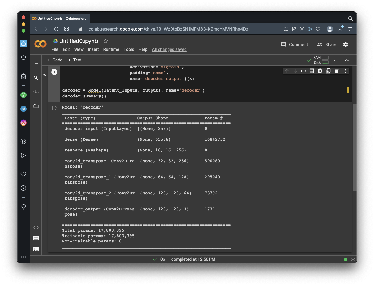
decoder = Model(latent_inputs, outputs, name='decoder')
decoder.summary()
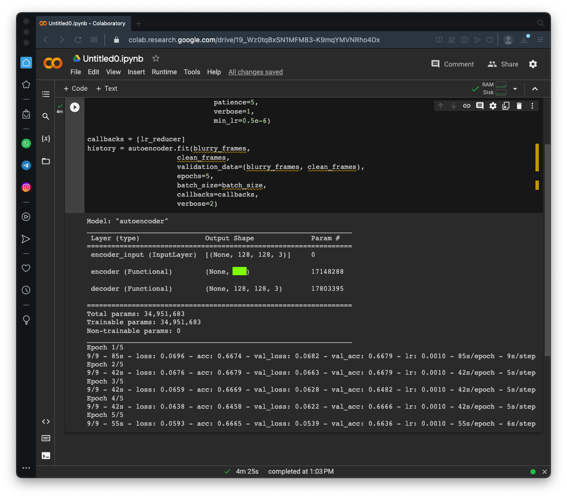
Flag ML 103.1: Training the Model (10 pts)
Execute this code to train the model:As shown below, the model has a total of 34 million parameters.autoencoder = Model(inputs, decoder(encoder(inputs)), name='autoencoder') autoencoder.summary() autoencoder.compile(loss='mse', optimizer='adam',metrics=["acc"]) lr_reducer = ReduceLROnPlateau(factor=np.sqrt(0.1), cooldown=0, patience=5, verbose=1, min_lr=0.5e-6) callbacks = [lr_reducer] history = autoencoder.fit(blurry_frames, clean_frames, validation_data=(blurry_frames, clean_frames), epochs=5, batch_size=batch_size, callbacks=callbacks, verbose=2)It will take about 5 minutes to go through 5 epochs of training.
The flag is covered by a green rectangle in the image below.
seed = 3
random.seed(seed)
np.random.seed(seed)

print("\n       Input                        Ground Truth                  Predicted Value")
for i in range(3):

    r = random.randint(0, len(clean_frames)-1)

    x, y = blurry_frames[r],clean_frames[r]
    x_inp=x.reshape(1,128,128,3)
    result = autoencoder.predict(x_inp)
    result = result.reshape(128,128,3)

    fig = plt.figure(figsize=(12,10))
    fig.subplots_adjust(hspace=0.1, wspace=0.2)

    ax = fig.add_subplot(1, 3, 1)
    ax.imshow(x)

    ax = fig.add_subplot(1, 3, 2)
    ax.imshow(y)

    ax = fig.add_subplot(1, 3, 3)
    plt.imshow(result)
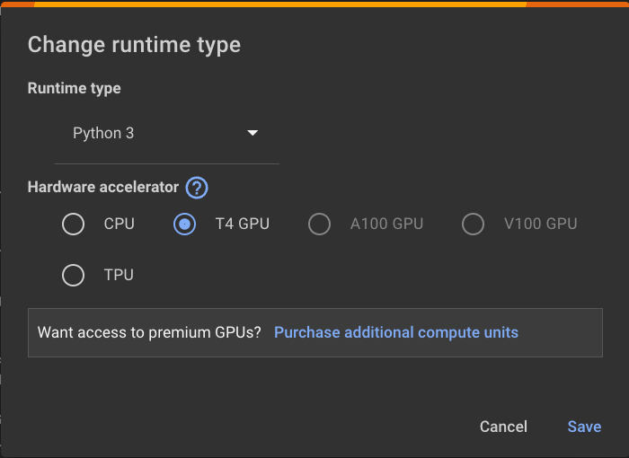
Click "Change runtime type".
Change the Hardware Accelerator to "T4 GPU", as shown below.
Click Save.
The training would have taken about 70 minutes using just the CPU, but with the T4 GPU, it only takes a few minutes.
Flag ML 103.2: Showing the Results (20 pts)
Execute this code to show the results.As shown below, the results are much better.seed = 3 random.seed(seed) np.random.seed(seed) for i in range(3): r = random.randint(0, len(clean_frames)-1) x, y = blurry_frames[r],clean_frames[r] x_inp=x.reshape(1,128,128,3) result = autoencoder.predict(x_inp) result = result.reshape(128,128,3) fig = plt.figure(figsize=(12,10)) fig.subplots_adjust(hspace=0.1, wspace=0.2) ax = fig.add_subplot(1, 3, 1) ax.imshow(x) ax = fig.add_subplot(1, 3, 2) ax.imshow(y) ax = fig.add_subplot(1, 3, 3) plt.imshow(result) print("Flag:", len(clean_frames)) print()The flag is covered by a green rectangle in the image below.
Flag ML 103.3: Smaller Dataset (10 pts)
Repeat the process using "blur2.zip" from my server. Be careful to change the folder name to "blur2" when fetching the good_frames and bad_frames.Train the model for 100 epochs.
View the results using the same code as for Flag ML 103.2.
As shown below, the results are pretty bad.
The flag is covered by a green rectangle in the image below.
Posted 4-13-23
Video added 4-20-23
Video updated 5-3-23
Import plot_model fixed 12-11-23, fixed more on 12-12-23
GPU instructions added 12-12-23
103.3 flag instructions expanded 7-22-24
Import added to "Prepare encoder", random seed fixed 12-12-24