ML 100: Machine Learning with TensorFlow (65 pts extra)

What You Need

A Web browser

Purpose

To practice making simple machine learning code in Python.

Using Google Colab

In a browser, go to

https://colab.research.google.com/

If you see a blue "Sign In" button at the top right, click it and log into a Google account.

From the menu, click File, "New notebook".

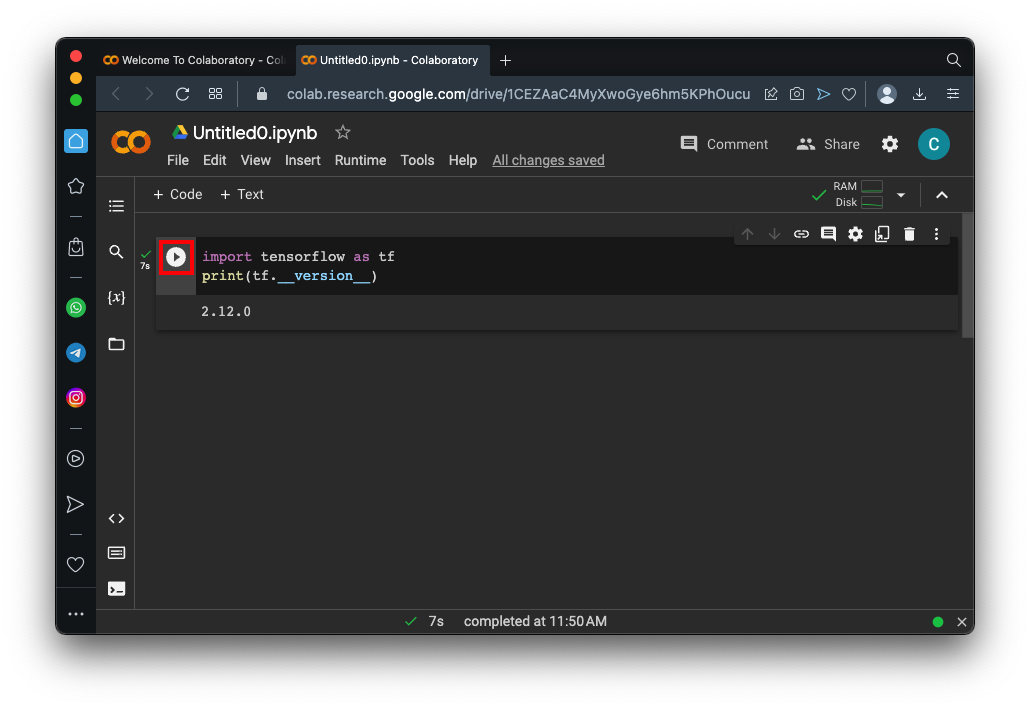
Enter this code:

import tensorflow as tf print(tf.__version__)

Click the Run button, outlined in red in the image below:

The tensorflow version appears, as shown above.

A Linear Relationship

Consider these numbers:

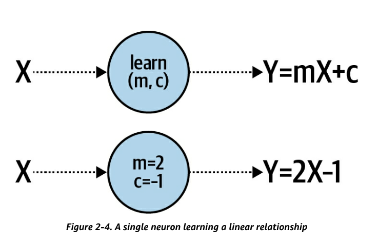
X = -1,  0, 1, 2, 3, 4
Y = -3, -1, 1, 3, 5, 7

Figure out the relationship between them. At first you can see that both numbers get larger, then you may notice that X increments by 1 and Y increments by 2, and figure out the relationship is:

Y = 2*X - 1

That's what scientists do with data--find relationships and describe them with math.

Machine learning figures out such relationships.

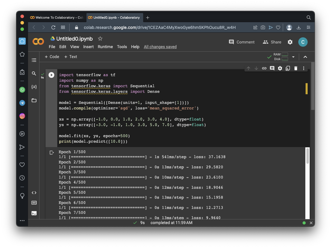
Machine Learning for a Linear Relationship

Enter the code below:

import tensorflow as tf import numpy as np from tensorflow.keras import Sequential from tensorflow.keras.layers import Dense model = Sequential([Dense(units=1, input_shape=[1])]) model.compile(optimizer='sgd', loss='mean_squared_error') xs = np.array([-1.0, 0.0, 1.0, 2.0, 3.0, 4.0], dtype=float) ys = np.array([-3.0, -1.0, 1.0, 3.0, 5.0, 7.0], dtype=float) model.fit(xs, ys, epochs=500) print(model.predict([10.0]))

Note these features of the code, which are explained more fully in chapter 1 of the Source book referenced at the bottom of this page.

The "model = Sequential..." statement defines a neural network with one layer, containing one node, and using input data with only one independent variable (X), as shown below. (Image from the textbook in the "Sources" at the bottom of this page.)
The "model compile..." statement tells it to use the "sgd" (Stochastic Gradient Descent) method to improve its rules, and to measure error by "mean_squares_error".

The ML program will guess at a relationship between X and Y, and measure how wrong it is by summing the square of all the errors.

It will then change its guess in the direction of lowering the error and try again.

Click the Run button.

As you can see, the "loss" number at the right end of each row is getting smaller. This is the error value.

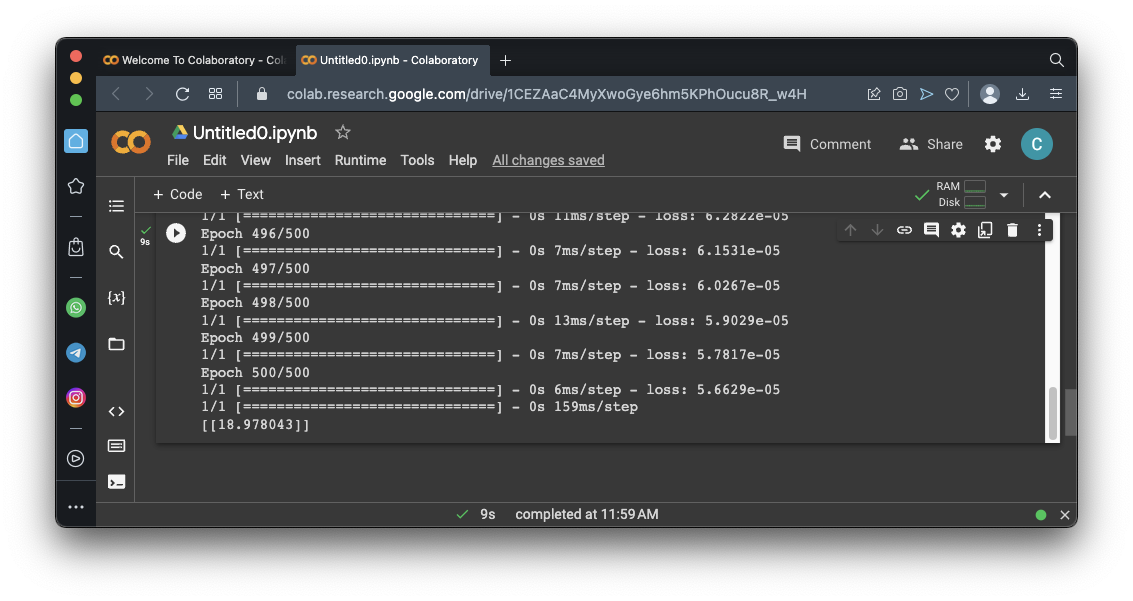
Scroll to the bottom of the output. As shown below, the error becomes very small, on the order of 10**-5.

At the end, it prints the model's prediction for Y when X is 10. The correct value is 19, and, as you can see, the model gets very close to it.

Seeing What the Network Learned

Enter the code below:

import tensorflow as tf import numpy as np from tensorflow.keras import Sequential from tensorflow.keras.layers import Dense l0 = Dense(units=1, input_shape=[1]) model = Sequential([l0]) model.compile(optimizer='sgd', loss='mean_squared_error') xs = np.array([-1.0, 0.0, 1.0, 2.0, 3.0, 4.0], dtype=float) ys = np.array([-3.0, -1.0, 1.0, 3.0, 5.0, 7.0], dtype=float) model.fit(xs, ys, epochs=500) print(model.predict([10.0])) 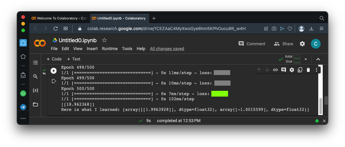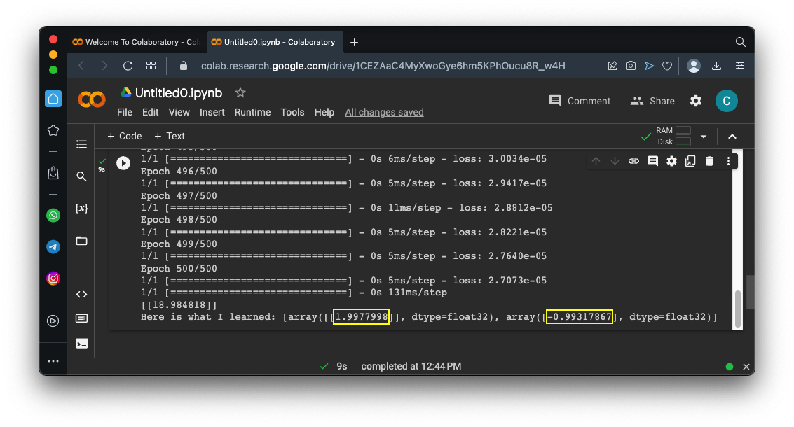print("Here is what I learned: {}".format(l0.get_weights()))

The variable "l0" holds the Dense layer, and at the end, we print out the weights, which are the estimated parameters connecting X to Y.

Click the Run button.

Scroll to the bottom of the output.

Remember that the correct relationship between X and Y is:

Y = 2*X - 1

Therefore, the first weight should be 2, and the second weight should be -1.

As outlined in yellow in the image below, the model gets very close to the correct weights.

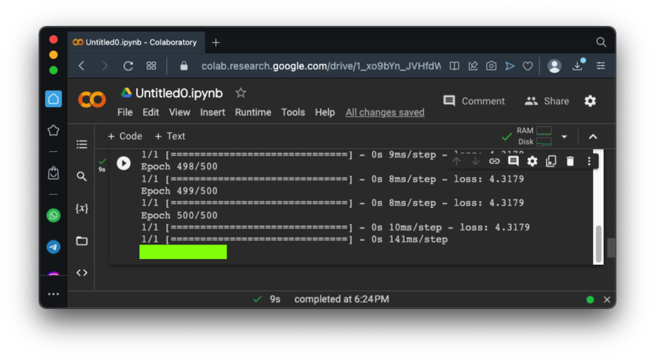
Flag ML 100.1: Learning with Errors (10 pts)
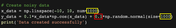
Change the "ys" line to the line shown below, which adds some random errors to the values:
ys = np.array([-3.1, -0.95, 1.07, 3.03, 4.91, 6.98], dtype=float)
The flag is covered by a green rectangle in the image below.

Flag ML 100.2: Fitting a Parabola (10 pts)
We'll use a parabola, defined by:
Y = x^2 -4*X - 5
Here are the calculated values: X Y -- -- -1 1 +4 -5 = -2 0 0 -0 -5 = -5 1 1 - 4 - 5 = -8 2 4 - 8 - 5 = -9 3 9 - 12 - 5 = -8 4 16 - 16 - 5 = -5 10 100 - 40 - 5 = 55
Change the "ys" line to the line shown below:
ys = np.array([-2, -5, -8, -9, -8, -5], dtype=float)
The correct answer is 55, but this model fails by a lot.
The flag is covered by a green rectangle in the image below.

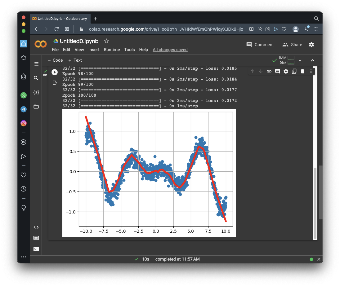
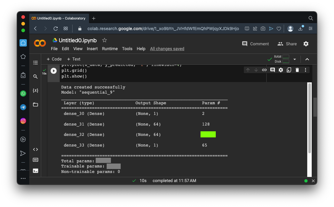
Flag ML 100.3: Fitting a Complex Curve (10 pts)
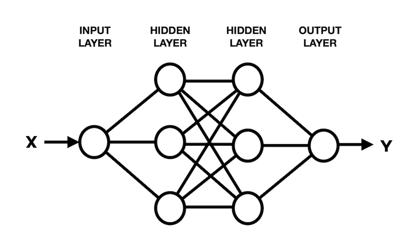
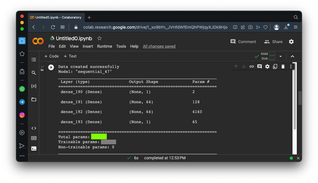
Run this model. It creates 1000 data points on a complex curve with noise, then creates a model with two hidden layers, then trains it and plots the results.
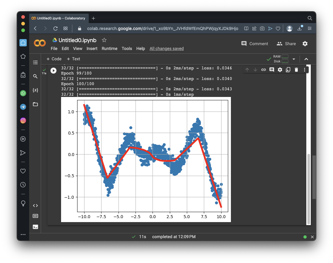
import numpy as np import matplotlib.pyplot as plt from tensorflow import keras from google.colab import files import tensorflow as tf import math # Create noisy data x_data = np.linspace(-10, 10, num=1000) y_data = 0.1*x_data*np.cos(x_data) + 0.1*np.random.normal(size=1000) print('Data created successfully') # Create the model model = keras.Sequential() model.add(keras.layers.Dense(units = 1, activation = 'linear', input_shape=[1])) model.add(keras.layers.Dense(units = 64, activation = 'relu')) model.add(keras.layers.Dense(units = 64, activation = 'relu')) model.add(keras.layers.Dense(units = 1, activation = 'linear')) model.compile(loss='mse', optimizer="adam") # Display the model model.summary() # Training model.fit( x_data, y_data, epochs=100, verbose=1) # Compute the output y_predicted = model.predict(x_data) # Display the result plt.scatter(x_data[::1], y_data[::1]) plt.plot(x_data, y_predicted, 'r', linewidth=4) plt.grid() plt.show()
You should see a red line, showing an excellent fit to the blue data points, as shown below.
Scroll up to the start of the output to see a diagram of the model. The flag is covered by a green rectangle in the image below.

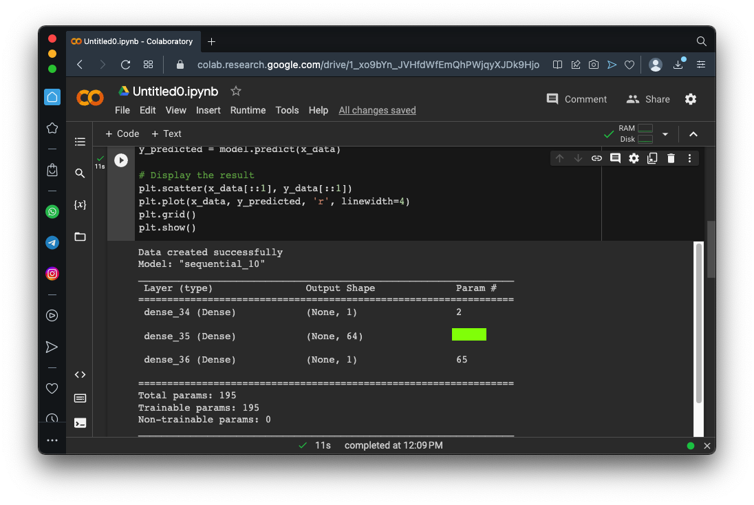
Flag ML 100.4: Using Fewer Layers (5 pts)
Run the model above, but add a "#" in front of one of these lines:
model.add(keras.layers.Dense(units = 64, activation = 'relu'))
The fit is still pretty good, as shown below.
Scroll up to the start of the output to see a diagram of the model. The flag is covered by a green rectangle in the image below.

Flag ML 100.5: Varying units and layers (15 pts)
Start with the code for ML 100.3, and run it with these variations:

32 units per layer, one hidden layer
16 units per layer, two hidden layers
4 units per layer, 3 hidden layers
4 units per layer, 4 hidden layers
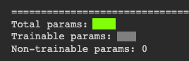
For each variation, run it three times and note the "loss" value for the fully trained model. Find the model with the lowest average loss after training--that's the best model.
Scroll up to the start of the output to see a diagram of the best model. The flag is covered by a green rectangle in the image below.

Flag ML 100.6: Varying input data and noise (15 pts)
Start with the code for ML 100.3. Notice lines of code shown below.
The number of points is 1000, outlined in yellow in two places.
The amount of noise is 0.1, outlined in red.
Try these combinations:

100 points, noise 0.1
1000 points, noise 0.5
300 points, noise 0.01
For each variation, run it three times and note the "loss" value for the fully trained model. Find the model with the lowest average loss after training--that's the best model.
Scroll up to the start of the output to see a diagram of the best model. The flag is covered by a green rectangle in the image below.

Sources

AI and Machine Learning for Coders: A Programmer's Guide to Artificial Intelligence
Different Types of Layers in Tensorflow.js
Neural networks curve fitting

Posted 4-10-23
Extra data removed from challenges 5 and 6 4-12-23
Video updated 4-20-23