Your First Machine Learning Project in Python Step-By-Step
python3 -m pip install scipy
python3 -m pip install numpy
python3 -m pip install matplotlib
python3 -m pip install pandas
python3 -m pip install sklearn
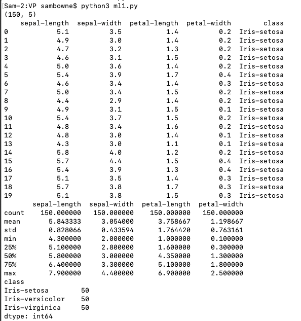
The data set contains 150 records of measurements of iris flowers.
Create a program named ml1.py containing this code:
from pandas import read_csv

# Load dataset
url = "https://raw.githubusercontent.com/jbrownlee/Datasets/master/iris.csv"
names = ['sepal-length', 'sepal-width', 'petal-length', 'petal-width', 'class']
dataset = read_csv(url, names=names)

# shape
print(dataset.shape)

# head
print(dataset.head(20))

# descriptions
print(dataset.describe())

# class distribution
print(dataset.groupby('class').size())
There are 150 records with 5 attributes. There are four measurements of each iris, sorted into three possible classes.
We want to write a program that will learn to identify the class of new irises from the other attributes.
# Load libraries
from pandas import read_csv
from pandas.plotting import scatter_matrix
from matplotlib import pyplot
from sklearn.model_selection import train_test_split
from sklearn.model_selection import cross_val_score
from sklearn.model_selection import StratifiedKFold
from sklearn.metrics import classification_report
from sklearn.metrics import confusion_matrix
from sklearn.metrics import accuracy_score
from sklearn.linear_model import LogisticRegression
from sklearn.tree import DecisionTreeClassifier
from sklearn.neighbors import KNeighborsClassifier
from sklearn.discriminant_analysis import LinearDiscriminantAnalysis
from sklearn.naive_bayes import GaussianNB
from sklearn.svm import SVC
# Load dataset
url = "https://raw.githubusercontent.com/jbrownlee/Datasets/master/iris.csv"
names = ['sepal-length', 'sepal-width', 'petal-length', 'petal-width', 'class']
dataset = read_csv(url, names=names)
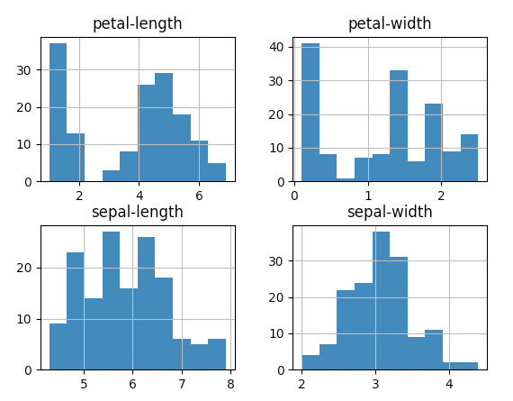
# histograms
dataset.hist()
pyplot.show()
The attributes "petal-length" and "petal-width" have two clear groups, suggesting that they may be important attributes to determine the class.
# Load libraries
from pandas import read_csv
from pandas.plotting import scatter_matrix
from matplotlib import pyplot
from sklearn.model_selection import train_test_split
from sklearn.model_selection import cross_val_score
from sklearn.model_selection import StratifiedKFold
from sklearn.metrics import classification_report
from sklearn.metrics import confusion_matrix
from sklearn.metrics import accuracy_score
from sklearn.linear_model import LogisticRegression
from sklearn.tree import DecisionTreeClassifier
from sklearn.neighbors import KNeighborsClassifier
from sklearn.discriminant_analysis import LinearDiscriminantAnalysis
from sklearn.naive_bayes import GaussianNB
from sklearn.svm import SVC
# Load dataset
url = "https://raw.githubusercontent.com/jbrownlee/Datasets/master/iris.csv"
names = ['sepal-length', 'sepal-width', 'petal-length', 'petal-width', 'class']
dataset = read_csv(url, names=names)
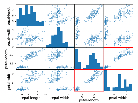
# scatter plot matrix
scatter_matrix(dataset)
pyplot.show()
These charts show relationships between the attributes.
For example, look at the two charts outlined in red in the image below. The dots lie close to a line, with little scatter.
This means there is a strong correlation between "petal-length" and "petal-width". That they both contain the same information--measuring one of them is enough to predict the other.
# Load libraries
from pandas import read_csv
from pandas.plotting import scatter_matrix
from matplotlib import pyplot
from sklearn.model_selection import train_test_split
from sklearn.model_selection import cross_val_score
from sklearn.model_selection import StratifiedKFold
from sklearn.metrics import classification_report
from sklearn.metrics import confusion_matrix
from sklearn.metrics import accuracy_score
from sklearn.linear_model import LogisticRegression
from sklearn.tree import DecisionTreeClassifier
from sklearn.neighbors import KNeighborsClassifier
from sklearn.discriminant_analysis import LinearDiscriminantAnalysis
from sklearn.naive_bayes import GaussianNB
from sklearn.svm import SVC
# Load dataset
url = "https://raw.githubusercontent.com/jbrownlee/Datasets/master/iris.csv"
names = ['sepal-length', 'sepal-width', 'petal-length', 'petal-width', 'class']
dataset = read_csv(url, names=names)
# Split-out validation dataset
array = dataset.values
X = array[:,0:4]
y = array[:,4]
X_train, X_validation, Y_train, Y_validation = train_test_split(X, y, test_size=0.20, random_state=1)
# Spot Check Algorithms
models = []
models.append(('LR', LogisticRegression(solver='liblinear', multi_class='ovr')))
models.append(('LDA', LinearDiscriminantAnalysis()))
models.append(('KNN', KNeighborsClassifier()))
models.append(('CART', DecisionTreeClassifier()))
models.append(('NB', GaussianNB()))
models.append(('SVM', SVC(gamma='auto')))
# evaluate each model in turn
results = []
names = []
for name, model in models:
kfold = StratifiedKFold(n_splits=10, random_state=1, shuffle=True)
cv_results = cross_val_score(model, X_train, Y_train, cv=kfold, scoring='accuracy')
results.append(cv_results)
names.append(name)
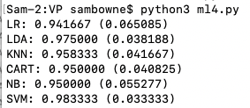
print('%s: %f (%f)' % (name, cv_results.mean(), cv_results.std()))
Your numbers will differ somewhat because the learning process contains some randomness.
The Support Vector Machines (SVM) model had the highest accuracy when I did it.
Flag VP 400.1: Load Data (10 pts)
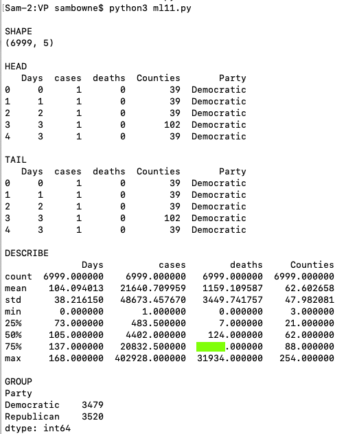
Download this file:COVID19c.csv(I made it from the sources listed at the bottom of this page. It is not perfect: I only identified 50 state governors, but there were 56 states in the raw case data. Please just regard it as random numbers for this project, not scientific evidence of anything.)Load the data and print summaries, as shown below.
The flag is covered by a green rectangle in the image below.
Flag VP 400.2: Best Model (10 pts)
Test the same six models on the data you downloaded in the previous challenge.Find the best model.
The flag is the name of that model, covered by a green rectangle in the image below.
Flag VP 400.3: Load Data (10 pts)
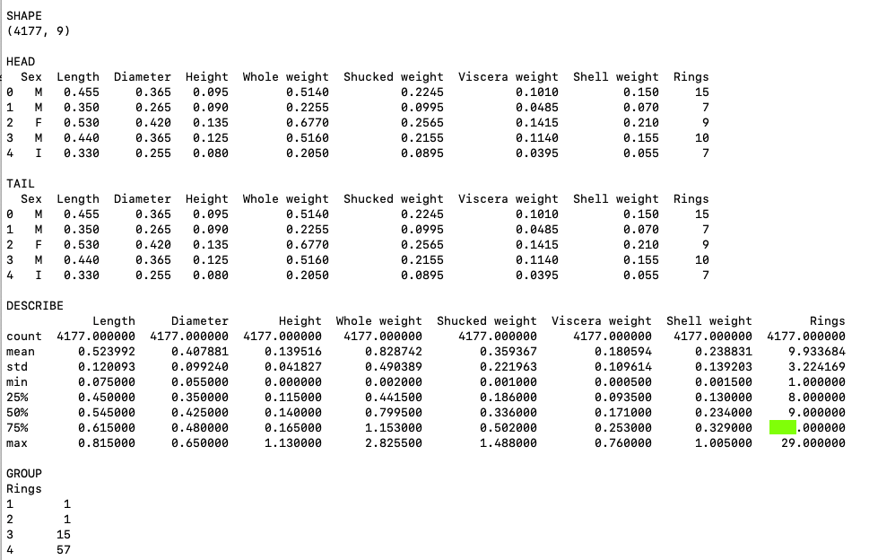
Download this file:Abalone.csv(I got it here.)Load the data and print summaries, as shown below.
The flag is covered by a green rectangle in the image below.
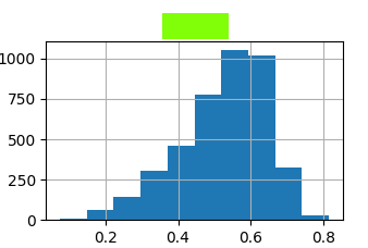
Flag VP 400.4: Histogram (5 pts)
Continue using the abalone data.What attribute has the histogram shown below?
The flag is the name of the attribute, covered by a green rectangle in the image below.
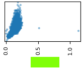
Flag VP 400.5: Multivariate Plots (5 pts)
Continue using the abalone data.Find the multivariate plot matching the image shown below.
The flag is the name of the attribute covered by a green rectangle in the image below.
Flag VP 400.6: Best Model (10 pts)
Continue using the abalone data.Remove the "Sex" column from the data.
Test the same six models on the data you downloaded in the previous challenge, using the other seven columns to predict "Rings".
Find the worst model. There are warnings that "The least populated class in y has only 1 members", as shown below, but just ignore them.
The flag is the name of that model, covered by a green rectangle in the image below.